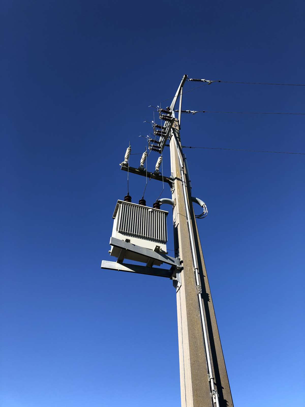
Transformers are very common devices, most of the time they go unnoticed and sometimes are hidden in plain sight. (click to enlarge)
Transformers are often treated at very simple components by ordinary electronics books: you just feed an AC voltage to its primary winding and a different voltage comes out at the secondary and the ratio of the voltages is the same as the ratio of the number of turns. Ok, often you also find information about what happens to the current and to the impedance, but very few texts talk more in detail about what really happens in a transformer. There are good theoretical books that address all the electromagnetism that happens inside from a theoretical point of view, but I always found this frustrating not to find a practical example.
Transformers are very common devices, most of the time they go
unnoticed and sometimes are hidden in plain sight. (click to enlarge)
So, on a rainy Sunday afternoon I decided to take a random transformer out of my junk-box and try to measure as many parameters as I could, just to put in practice the theory I learned in school many years ago, but never had a chance to experience. Seeing if the theory corresponds to the practice is an excellent occasion to better understand this kind of mysterious electronic component. At least this seemed like a good thing to do on a rainy day. It turned out that it was a very deep rabbit hole that took many afternoons; actually, there were a multitude of rabbit holes that took a lot of afternoons to explore, and I could still play with it some more.
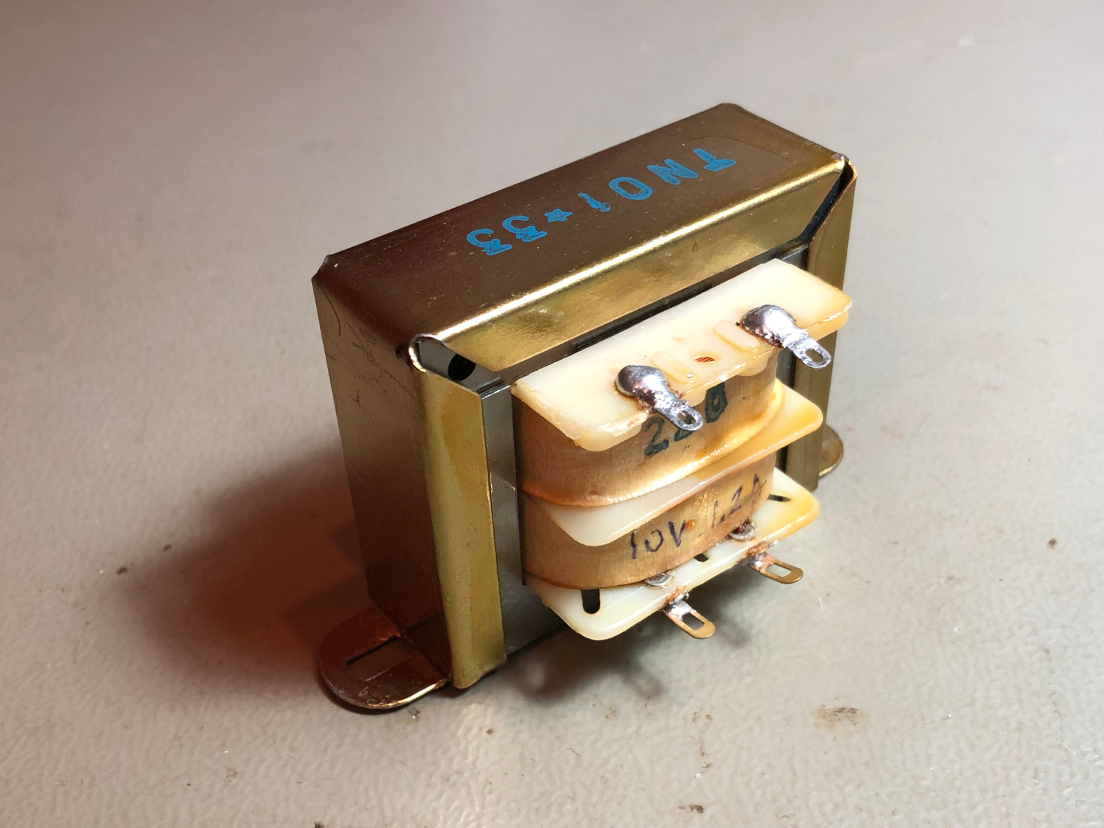
The victim of our measurements, a small transformer out of my junk-box
labelled TN01-33. (click to enlarge)
The victim that came out of the junk-box is a small E-I core transformer labelled TN01-33, probably made by Stelvio in Milan (Italy) back in the '80s. I could not find any datasheet nor a vintage catalogue, but I remember it was used by Nuova Elettronica (an Italian electronics magazine) in its kits, and this is likely how it ended up in my junk-box. I could find it was used in the LX.1044 kit that was published in magazine N.150 in September 1991: in that article it was rated 220/10V, 1.2A, 15VA. Without being explicitly written, this transformer is intended to work with a mains frequency of 50Hz.
Our transformer is quite small: its core measures only 57×47×18mm3 and is composed of an E-I stack of 36 steel sheets of a thickness of 0.5mm. It weighs 410g.
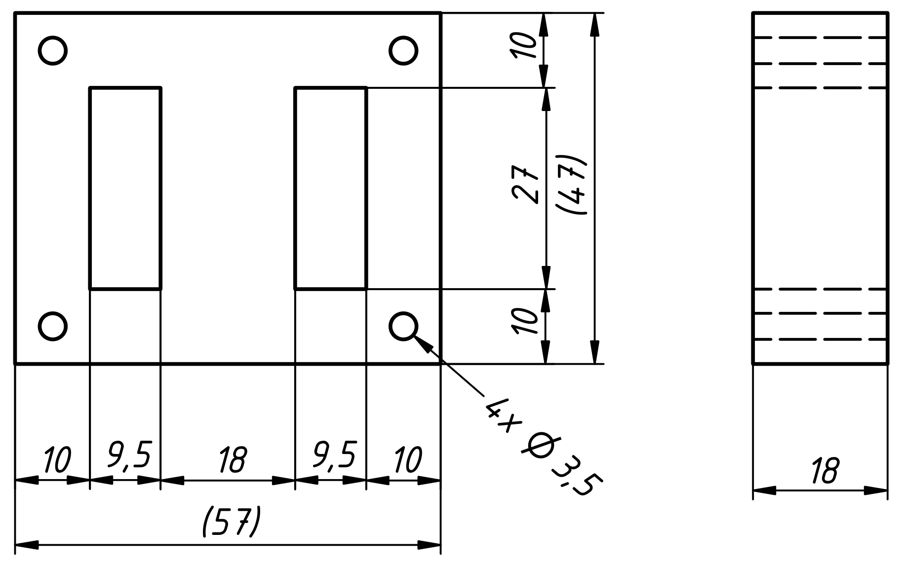
Mechanical dimensions of the core. (click to enlarge)
As shown in the figure below, the core cross section S is 18×18mm2 = 324mm2. This is just the area of the central section of the core, because all the flux goes through this section and then splits in half and loops through the two side sections which have roughly the same area when combined.
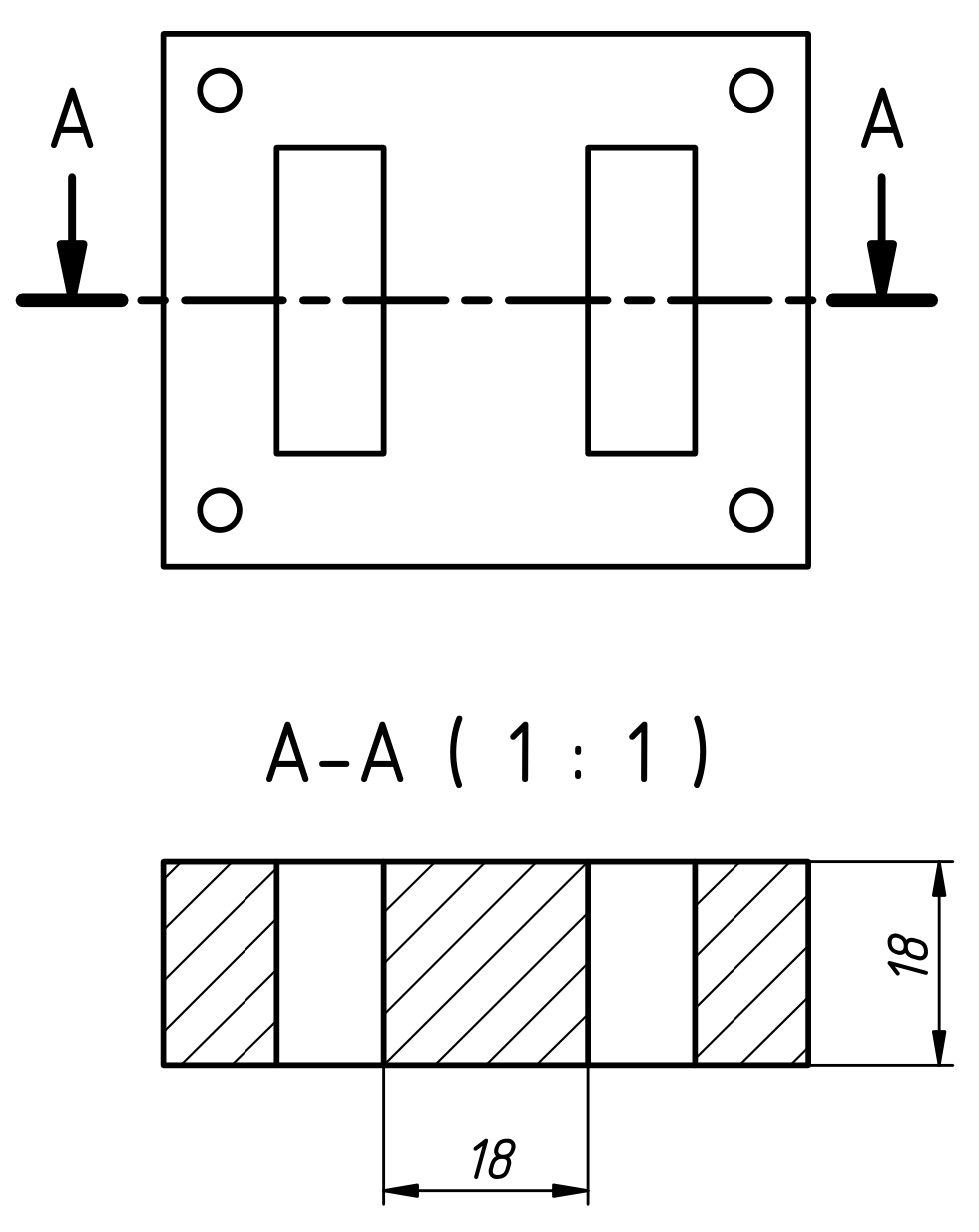
Cross section and mechanical dimensions of the core.
The middle section goes through the windings and measures
18x18mm2. (click to enlarge)
The power of a transformer is not theoretically a function of its cross-section, but there is a practical rule of thumb [1] that considers how much iron is usually necessary to accommodate the copper of the windings and is very handy when salvaging an old transformer of unknown characteristics.
The material of the core is not known, so it is supposed to be the cheapest transformer steel available that has an efficiency η of about 80%. By using the said rule of thumb, we find:

We just found that this transformer (apparent) power should be 5.4VA. This is quite strange, as the transformer is supposed to be 15VA... Something isn't quite right.
This is something I learned by playing with this transformer: cheap and small transformers are often built with a smaller core and with fewer turns. The core saturates and has higher losses, but the transformer still works and is cheaper. Only heavy-duty transformers have the correct amount of metal and minimize losses. This unexpected saturation fooled me and made me redo the measurements many times until I could finally figure out what was wrong. The next time a see a small core compared to its rated power it will ring me a bell and save me quite some time.
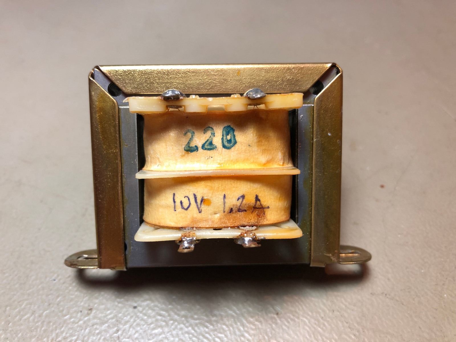
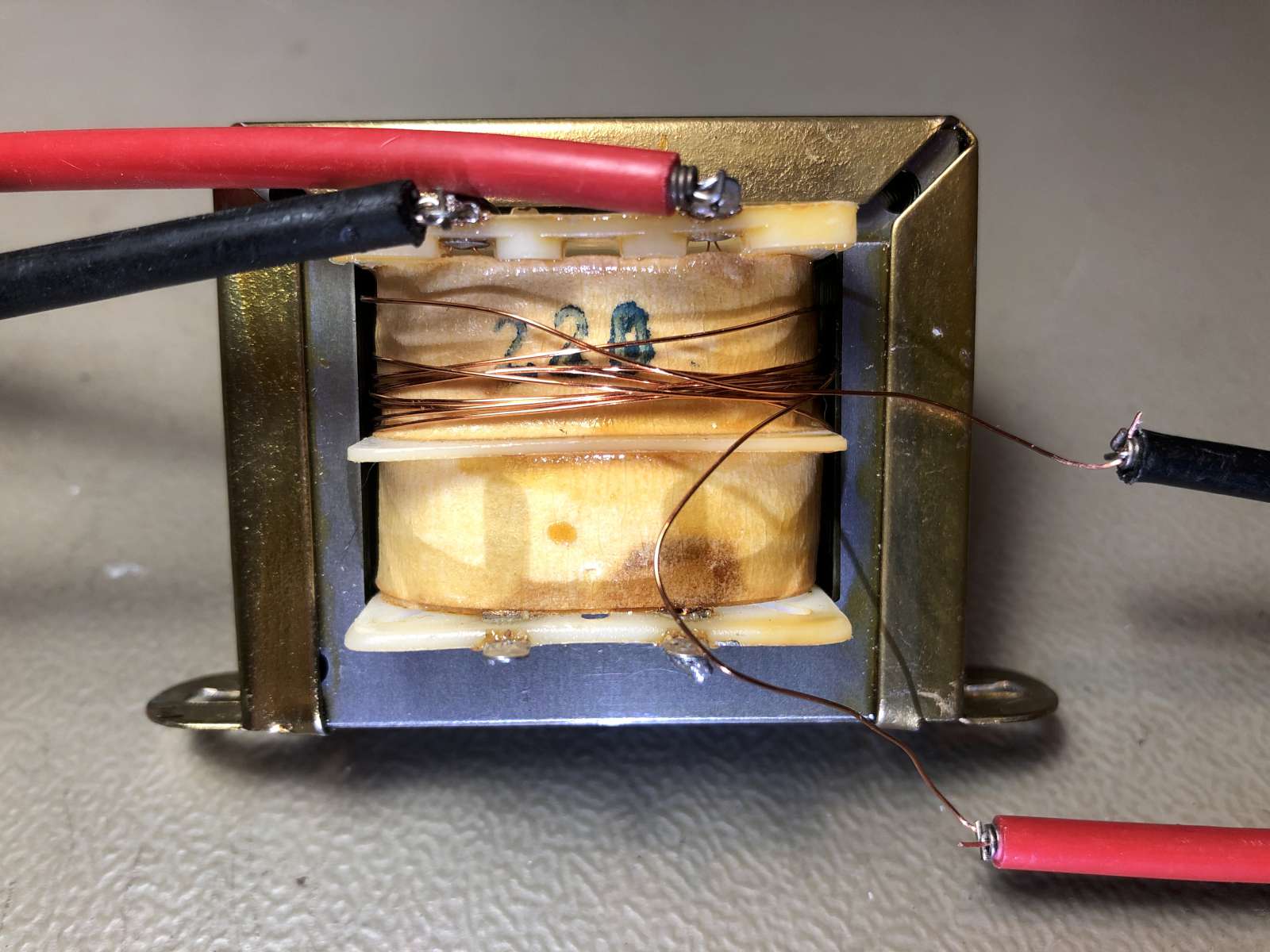
Front view of the transformer.
The Shape of the core and the position of the two windings is clearly
visible. Luckily the manufacturer stamped "220" on the primary side
so I don't have to figure out the primary voltage. (click to enlarge)
Now that we know something about the core, let's do some theoretical calculations to determine how many turns we should wind if we had to build this transformer from scratch.
Let's suppose a flux density %phi; of 1.0Wb/m2 which is a good approximation for a cheap steel core, a mains frequency f of 50Hz and calculate how many turns per volt such a core would require:

From this, we expect a primary winding with 3'057 turns and a secondary one of 139 (or 146 if we compensate for 5% of coupling losses). The turns ratio ü should be, of course:

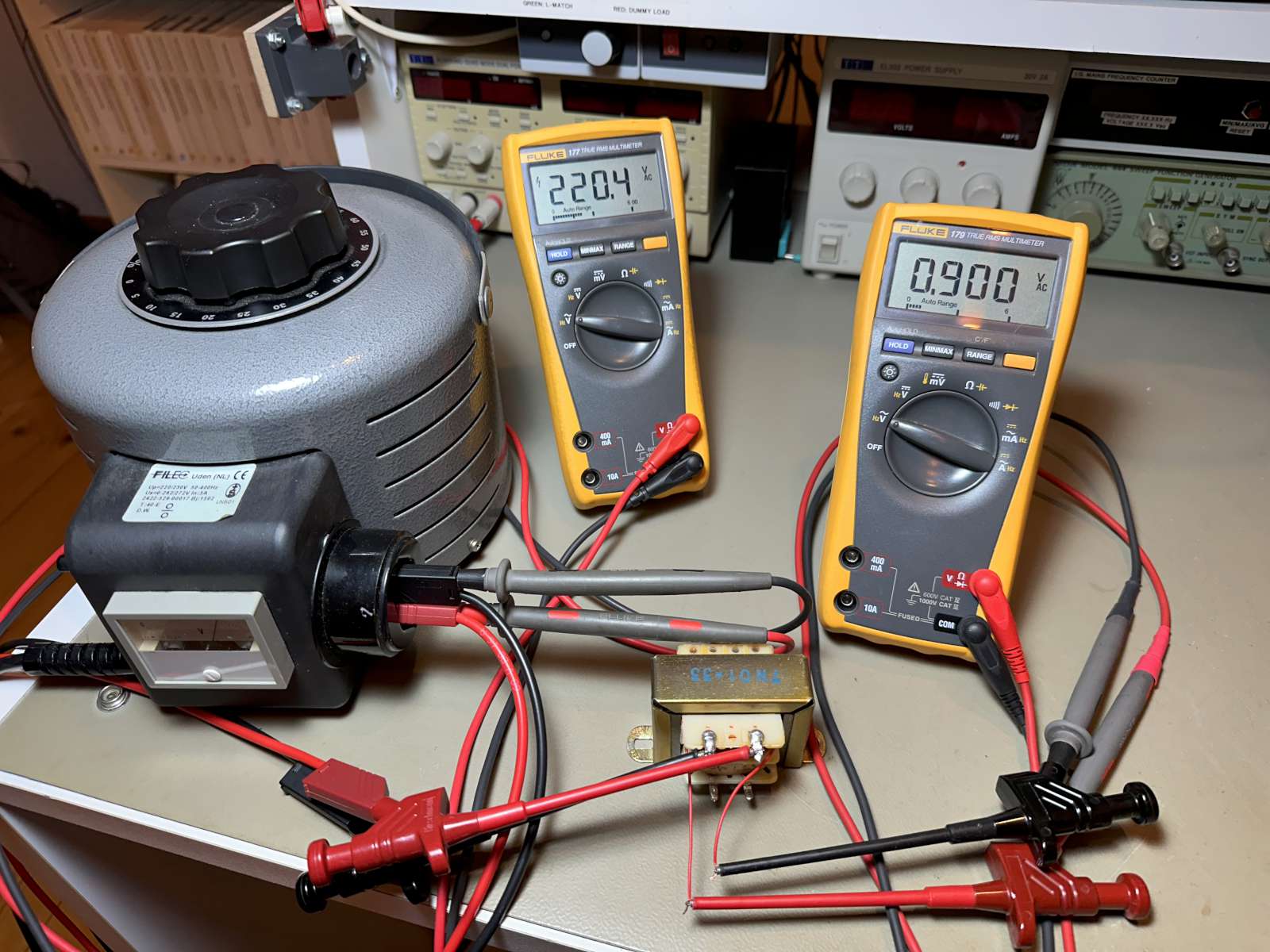
Let's verify this in practice. Let's connect the transformer to the mains and measure its turns ratio. Since the primary is clearly marked by the manufacturer and the voltages are known, no special precaution is needed.
For sake of accuracy, I used a variac to adjust the mains voltage to about 220V for this measurement. This is because the mains voltage today is no longer 220V as it was in the '80s: officially it's now 230V but is usually closer to 240V in the region I live in. This later turned out to be unnecessary as the voltage ratio stays very constant over the full voltage range.
With a primary voltage Up of 220.0V the secondary voltage Us reads 10.94V. The frequency f is 50.0Hz. We can therefore calculate the turns ratio ü = 20.1:1. This isn't 22:1. The real voltage ratio is always smaller due to leakage inductances. I usually increase the number of turns of the secondary by about 5%, but here we have 8.6%: this is another clue that this transformer may be lossy because of its small core. The secondary voltage is kept a bit higher to account for losses when the transformer is loaded.
Let's see what happens when the transformed is used in the other way around. So, I connected a source of 12.04V to the secondary and measured the voltage on the primary to be 236.3V. The turn ratio in the reverse direction is 19.6:1. This transformer definitely has a nominal turns ratio around 20:1 rather than the expected 22:1.
To have a better understanding, let's wind a few turns on the core and find out how many turns the windings actually have.
Determining the number of turns with an auxiliary winding.
(click to enlarge)
We build a test wining of Nt = 9 turns around the core and we measure a voltage Ut = 0.900V across it when the primary voltage is 220.4V. We can now calculate that this transformer has a constant γ = 10.00 turns per volt. From this, we can estimate that the primary has Np = 2'200 turns and the secondary has Ns&nbps;= 110 turns. This supposes that the coupling is 100%, which is not exactly true, but gives a better idea of the real number of turns than the previous estimation only based on the core cross section.
In other words, this tells us that this transformer is designed to be cheap because has less turns than it should. We determined that this core required 13.89turns/V but it only has 10. We expected the primary of having 3'057 turns but it only has 2'200. We therefore expect some core losses and a transformer that runs a warm due to the higher flux in the core: this is definitely not a heavy-duty component.
Not surprisingly, saturation is found in a later test. By the number of turns we can estimate that the designers, instead of 1.0Wb/m2, went for a flux of 1.4Wb/m2 that gives exactly 10 turns per Volt, deliberately saturating the core to save copper and iron (and cost).
We know that the core saturates. Does the transformer ratio stay constant, or does it change with saturation? To find out, let's do some measurements for different primary voltages. With the variac I have, I can sweep voltages from a few Volts up to 280V.
The result is a nice straight line, and the voltage ratio is fairly constant over the whole voltage range.
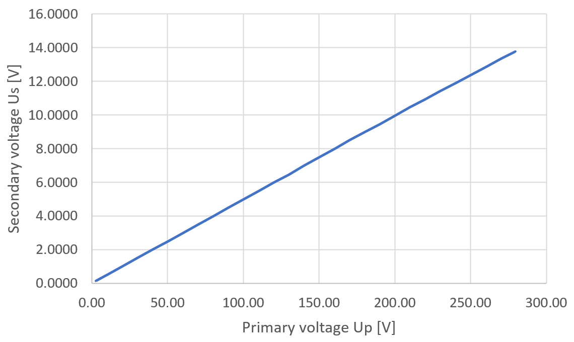
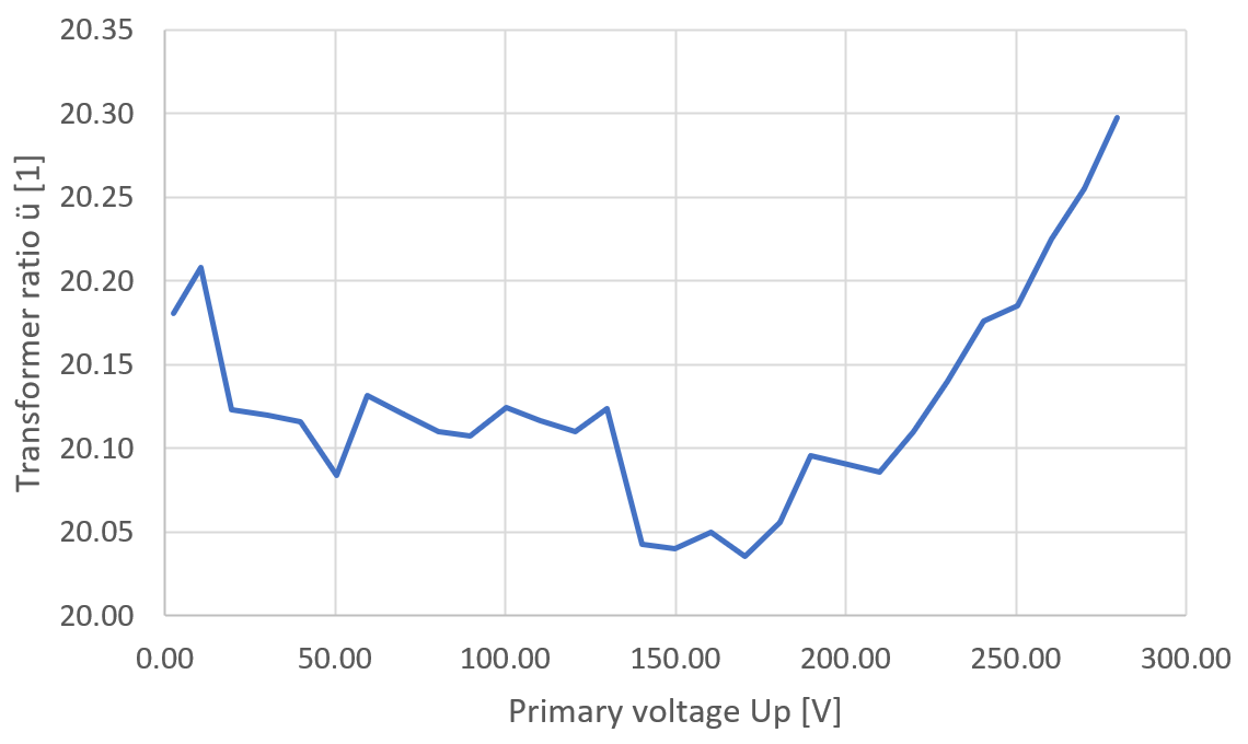
Secondary voltage (left) and transformer ratio (right) as a function
of primary voltage. (click to enlarge)
Measuring the turn ratio. (click to enlarge)
Let's now have a look at inductances and coupling factors to figure out the transformer equivalent circuit. By measuring the winding inductance alone and then by connecting them in series it's possible to determine the coupling factor of the transformer.
But this is easier said than done. Measuring the inductance of the coils turned out to be very, very tricky.
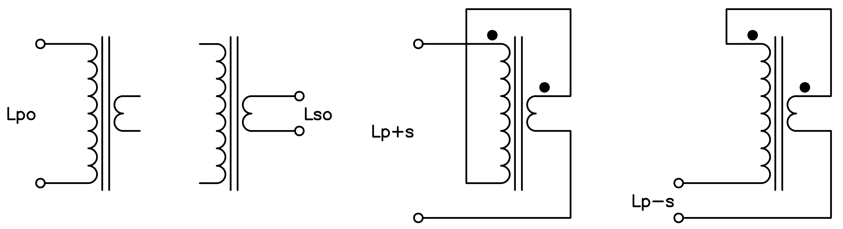
Inductances of the primary and secondary windings: each one alone,
both in series and both in anti-series. (click to enlarge)
The figure above explains how the measurements are made and the results are summarized in the table below:
| Primary inductance, secondary open | Lpo = 16.229H |
| Secondary inductance, primary open | Lso = 0.04924H |
| In-phase series inductance | Lp+s = 17.462H |
| Counter-phase series inductance | Lp−s = 14.964H |
Windings can be connected in-phase or in counter-phase. When connected in-phase (Lp+s) not only the two inductances add up, but the mutual inductance also increases the total inductance:

With this formula, we can determine the mutual inductance:

To get the coupling factor, we use the formula:

And we find:

Which is quite low, as I was told good transformer have a coupling close to 1.
Measuring Lp+s pleaseenote the short wire connecting
the two windings. (click to enlarge)
As verification, we can do the same calculation when the coils are connected in counter-phase (Lp−s). The two inductances add up, but the mutual inductance decreases the total inductance, and we have:

This time we found:

Which is higher than before. The coupling factor is calculated in the same way, and we get:

It would be better to find the same value with both measurements, but this was not the case, unfortunately. We can only conclude that the actual values are probably somewhere in the middle: say Lm is 625mH and k is 0.7.
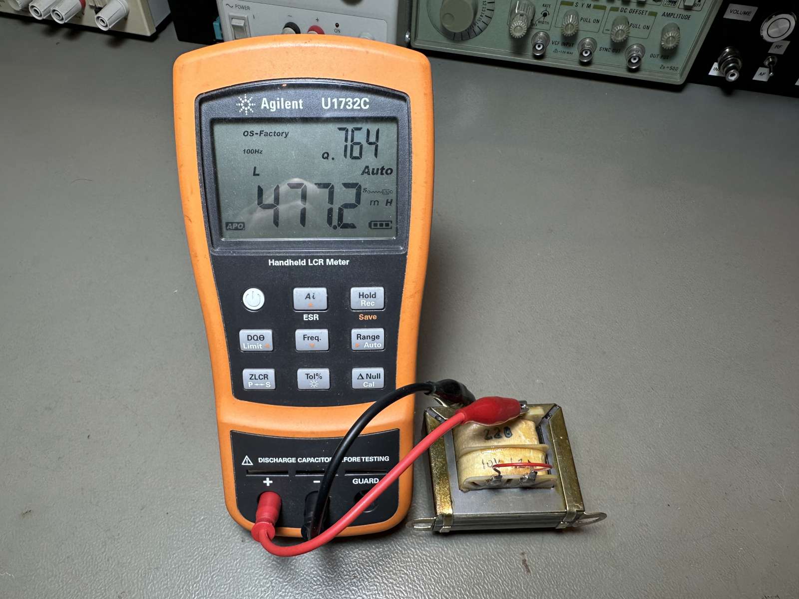
I did the same measurements over and over with many different inductance meters. The precision of the measurement is of paramount importance as the formula involves a very high value (16.229H) and a low one (0.04924H): small errors have a significant impact on the result. Not all inductance meters can measure large inductances accurately: most of them can read μH and mH, but cannot read H. Furthermore, the frequency at which the inductance is measured also has a large impact: too low and the core will saturate, too high and the core will act as a shorted winding.
I finally ended up trusting the readings from an Agilent U1732C as it was the only one capable of measuring all these inductances at a frequency of 100Hz, which is the closes I could get to the nominal 50Hz of this transformer. In my investigation I also used a Juntek LC-200A (had trouble reading low inductances), a UNI-T UT8803E (also had troubles reading low inductances) and a Voltcraft LCR-9063 (that was way off in high inductances).
Furthermore, when measuring inductances, one should make sure the core is not magnetized. If it is, its permeability would be lower and results will be lower, too. I repeated the measurements several times in different occasions and got inconsistent results. Only after accurately degaussing the core, I could get consistent (and higher) readings. To degauss the core, the primary is connected to a variac and the voltage is slowly decreased from 230V down to zero, the secondary is left open.
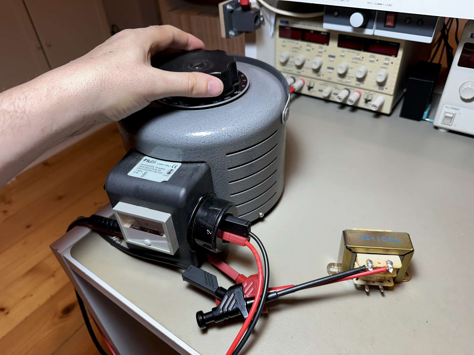
Degaussing the core. (click to enlarge)
The test winding composed of 9 turns of enameled copper wire coiled
over the primary winding (re-wound with a different wire for the picture).
(click to enlarge)
Before, we have added a temporary test winding to try to determine the number of turns: we can also measure its inductance while all other windings are open, as illustrated below:
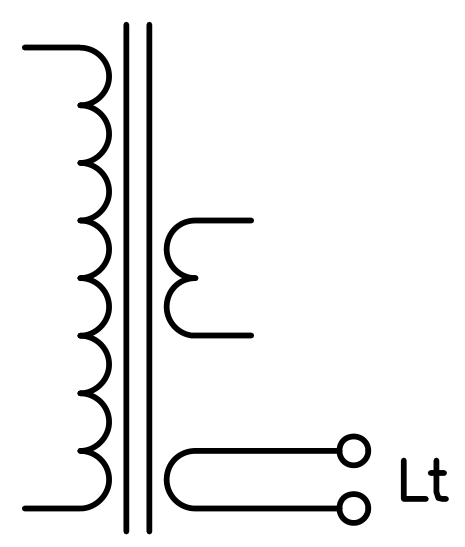
Test winding inductance measurement. (click to enlarge)
This is extremely tricky to measure: Commercial inductance meters use frequencies way too high for the core and only see a few μH. In the MHz range the core acts as a shorted winding and the result is largely underestimated. When measuring the impedance at 50Hz one must use a very low voltage to keep the core out of saturation and there is a lot of noise in the result.
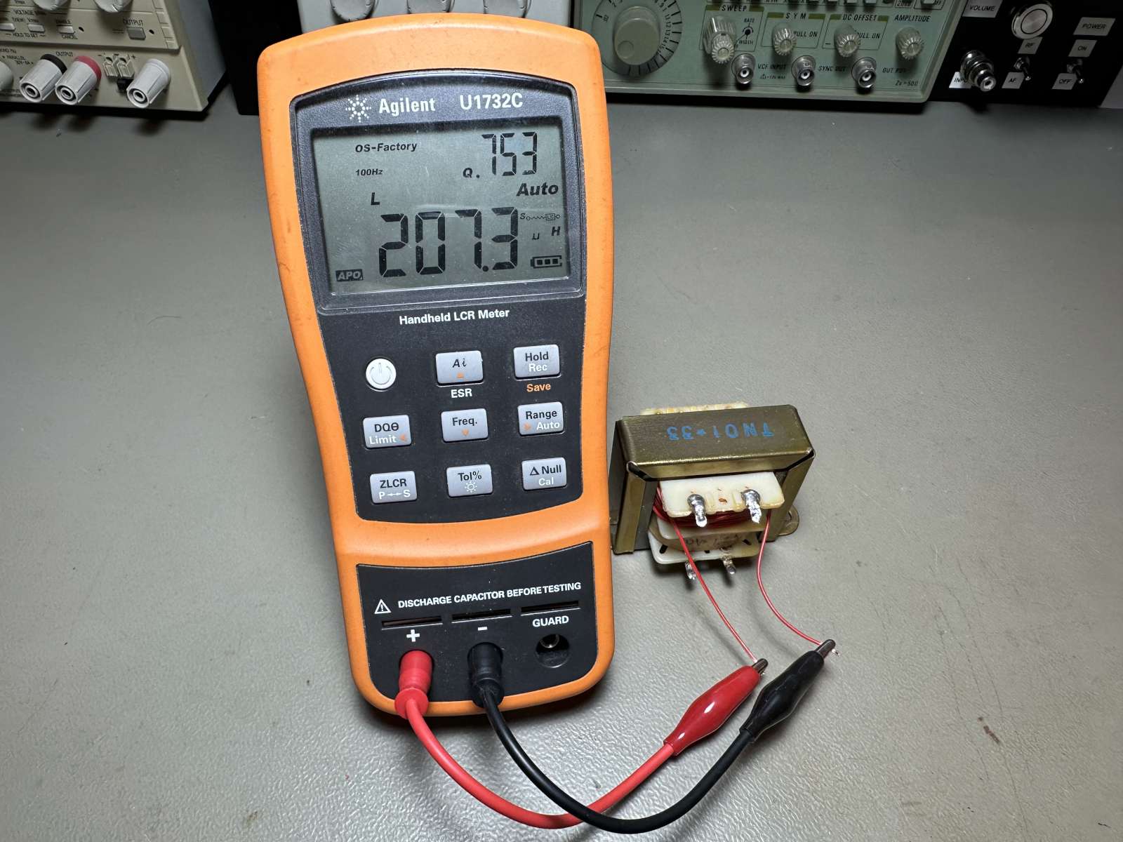
Measuring the inductance of the test winding. (click to enlarge)
At the end we found Lt = 207.3μH. Since we know the number of turns Nt = 9 we can calculate the inductance factor AL (or core nominal inductance or inductance per square turn) of the core:

From this value, we can estimate the number of turns of the windings:

and

These figures are a little different from what we have found before with simply the voltage ratio. We can also recalculate the turns ratio ü' = 18.2:1. It's true that these values don't depend on the coupling factor, which can introduce some errors, but they depend on inductance measurements that come with their dose of inaccuracy and show significant differences when the core saturates. So, I'm quite happy that ü' is not too far off from the 20.1:1 we found before, but I trust the 20.1:1 as the accuracy is much better.
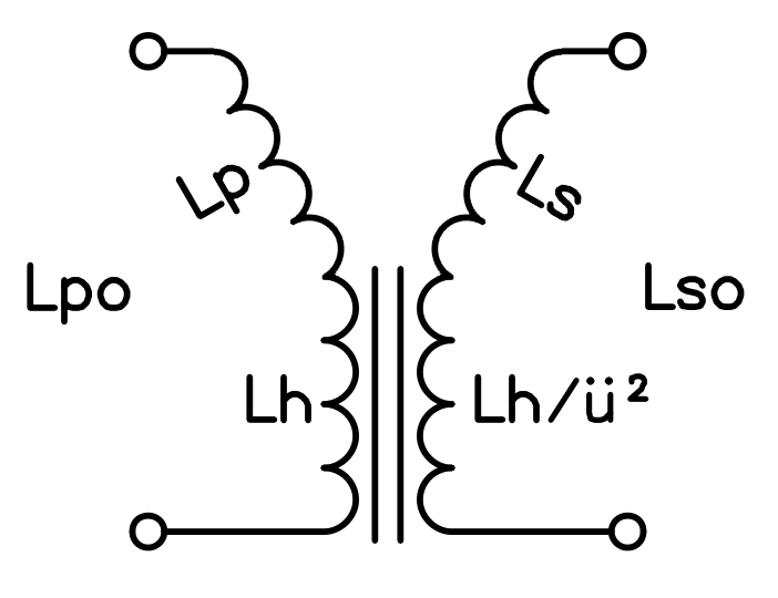
A transformer is difficult to model because of the mutual induction the couples the windings together. Hopefully, there is an equivalent circuit that is much easier to model or calculate, where mutual inductions are replaced with simple "regular" inductors without any coupling. The transformer ratio is modeled with an ideal transformer that simply scales current up and voltages down. The beauty of this circuit is that it works for any kind of signal: sinusoidal and not. The only condition is that the core must not saturate (everything must be linear).
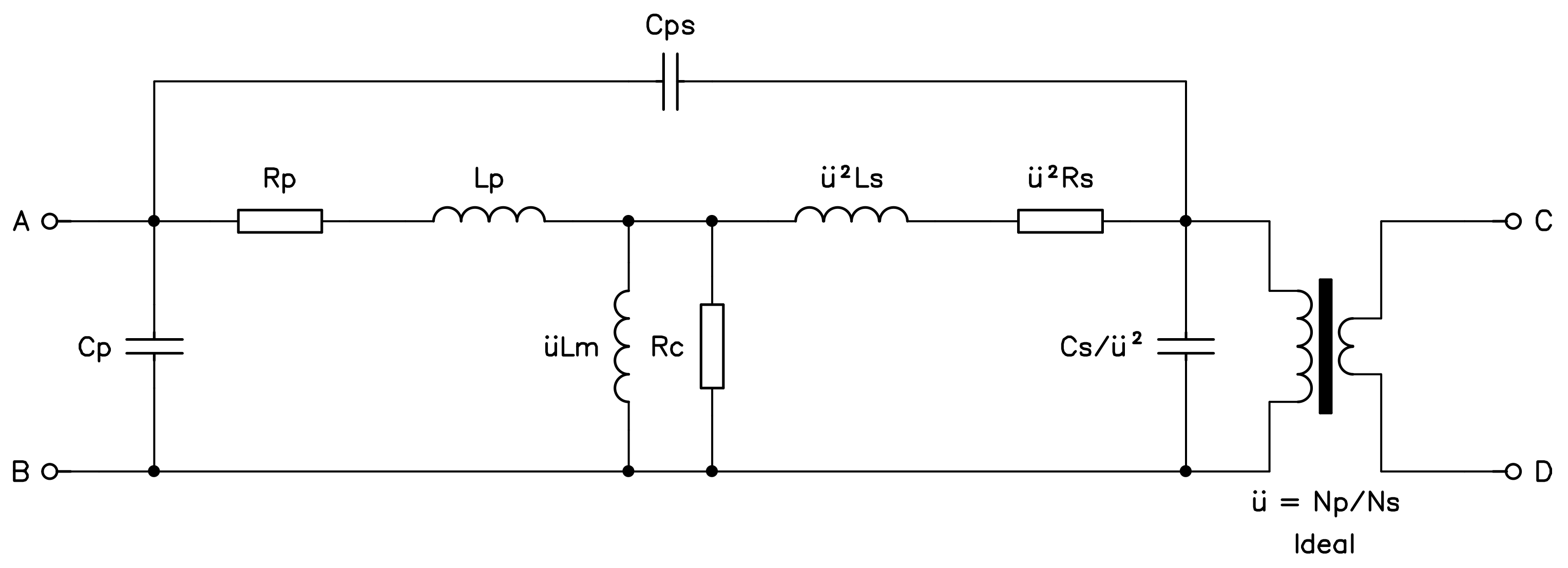
General transformer equivalent circuit.
In this circuit, there is no coupling anymore, just regular uncoupled
inductors, resistors, and capacitors.
The ideal transformer on the right just scales the current and the voltage,
but has no inductance, no resistance, and no capacitance.
(click to enlarge)
We know that our core saturates, so the model won't be accurate, but let's see if we can still do it just to explore the method of measuring and calculating these parameters. For this, we must perform some more measurements. So far, we have only measured the inductance of a winding when the other winding is left open. If we place a short circuit on the other winding, we measure a much smaller inductance. This is easy to see in the equivalent circuit, because shorting out one winding is equivalent of shunting Lh with another inductor of much smaller value. By the way, Lh is called magnetizing inductance (or main flux inductance) and is simply the mutual inductance multiplied by the transformer ratio.

The magnetizing inductance Lh is usually very large. It's what limits the current when the transformer is connected without load. When a winding is short-circuited, Lh is almost short circuited as well and only the leakage inductances are left in the circuit. Ideally the inductance seen from one winding should drop to zero if the coupling factor was 100%: in this case there are no leakage inductances.
I initially thought that measuring inductance values while shorting the other winding was necessary for calculating the leakage inductances. It turned out that it wasn't necessary as the mutual inductance was enough; still, I find interesting to see what happens when a winding is shorted and how well this transformer model explains it.
A representation of leakage inductances Lp and
Ls: they act as series inductances but don't participate to
the transformer action. (click to enlarge)
One can imagine leakage inductances as series inductances that are not magnetically coupled and don't participate to the transformer action as the mutual inductance does.
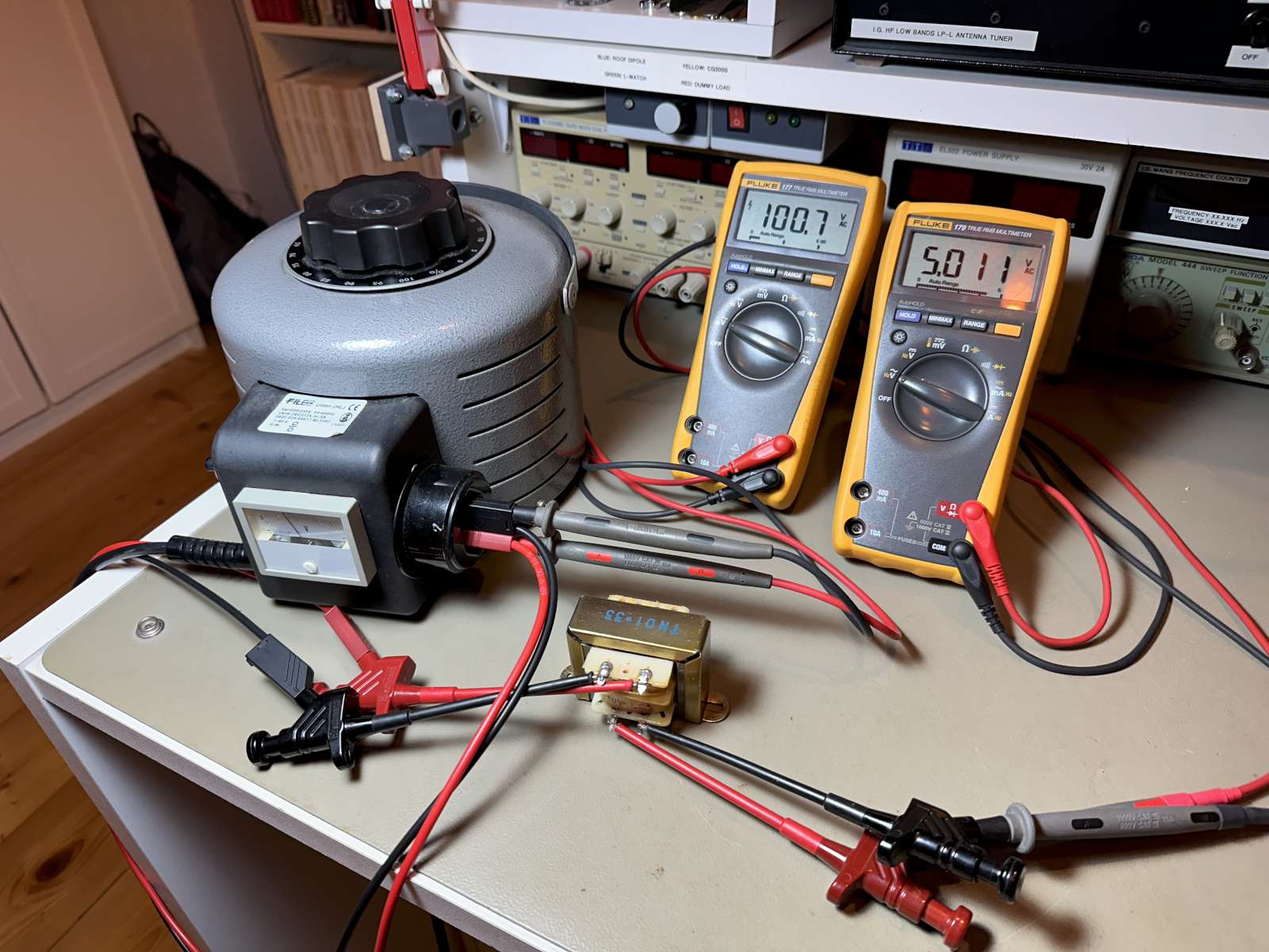
Now, back to our transformer and let's do some measurements:
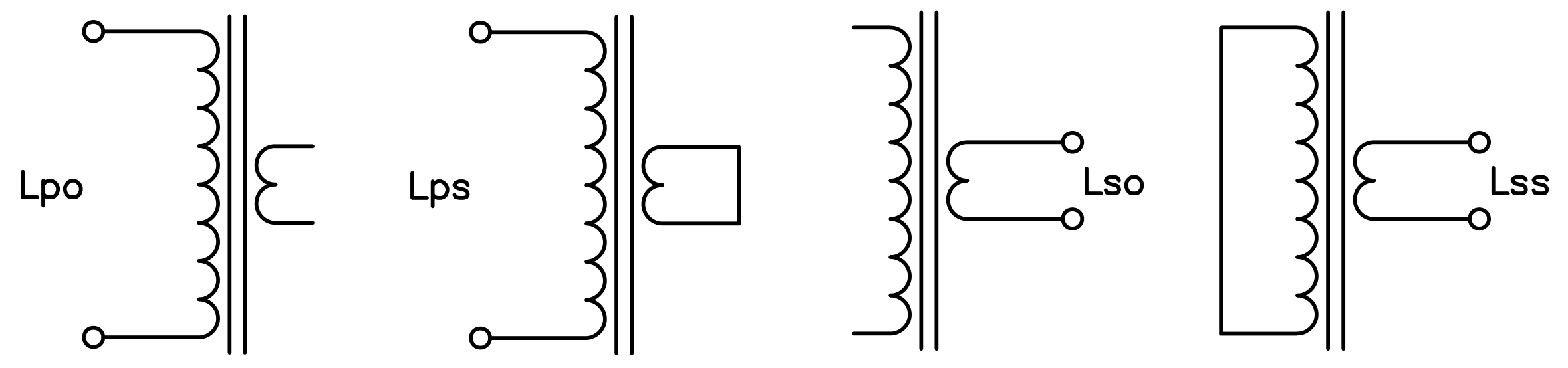
Measuring winding inductance of one winding while the other one is
open or short-circuited. (click to enlarge)
The figure above illustrates how these measurements are done and the results are summarized in the table below:
| Primary inductance, secondary open | Lpo = 16.229H |
| Primary inductance, secondary shorted | Lps = 477.2mH |
| Secondary inductance, primary open | Lso = 49.24mH |
| Secondary inductance, primary shorted | Lss = 1.1911mH |
Measuring the primary inductance while the secondary is shorted.
The result is a much smaller value because the large value of
üLm is shorted out by the much smaller
ü2Ls. (click to enlarge)
We already determined the mutual inductance Lm = 624.5mH (average of the two values found from Lp+s and Lp−s) and the transformer ratio ü = 20.1:1 (determined when measuring the voltage as the one from the inductances is less accurate). We can now calculate the magnetizing inductance or main flux inductance Lh:

By looking at the equivalent circuit, we see that if the secondary is open, Lpo = Lp+Lh, where Lp is the primary leakage inductance, and we can calculate Lp:

The primary leakage inductance Lp should not be confused with the primary inductance (with the secondary open) Lpo: the first one is a measure of how leaky the transformer is, i.e. how much it behaves like a simple inductor and not like a transformer and is usually quite small. The second one is what you measure when the other winding is not connected and is usually a very large value because you see the leakage inductance and the magnetizing inductance together, connected in series. In other words:

The same remark applies also to the secondary winding, but the secondary is a little trickier. In the model, all the components are moved on the primary side. When we measure the secondary inductance, we observe the transformer from the other side and the transformer ratio is reversed; from the secondary we don't see ü but 1/ü. So, the main flux inductance L'h as seen from the secondary side is:

With this, we can compute the secondary leakage inductance as seen from the secondary side:

Finally, we can calculate the secondary leakage inductance Ls as seen from the primary by multiplying by ü2:

Again, we are dealing with equation where large and small values are mixed together: beware that small errors in the measurements can lead to large errors or even inconsistencies in the result. Make sure that all your measurements are accurate and double check if the results make sense: it's very easy to end up with some nonsense such as a negative inductance.
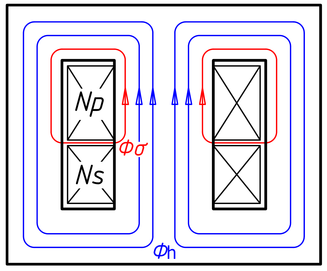
Main flux Φh and leakage flux
Φσ in our core. (click to enlarge)
The figure above illustrates the main flux Φh in blue and the leakage flux of the primary Φσ in red. As one can see, the leakage flux does not go through the secondary. Of course, there is also a leakage flux of the secondary that is not illustrated here.
Leakage in a transformer is not always a bad thing and sometimes it's desired. It doesn't directly cause losses but reduces the coupling factor, the transformer ratio (sometimes) and increase leakage inductance. If leakage is high, one can image that a significant part of the turns are not coupled together, they don't take part to the transformer action but simply behave as series inductance. This is desired in many applications, especially when the transformer must limit the current on its secondary, like in an arc welder, in a neon sign transformer, in a sodium-lamp ballast, in a microwave oven transformer,... Higher (or adjustable) leakage is achieved with longer cores and magnetic short-circuits. These are iron bars that are inserted into the core to provide a magnetic path around the primary diverting some of the flux out of the secondary.
Winding resistances Rp and Rs can directly be measured with an Ohm-meter (multimeter) as DC resistance is a very good approximation of what happens at 50Hz: we find Rp = 194.87Ω and Rs = 0.490Ω. To accurately measure low resistance values a 4-wire measurement was used. But a simple 2-wires measurement can also be used if one subtracts the resistance of the test leads, but the accuracy is lower.
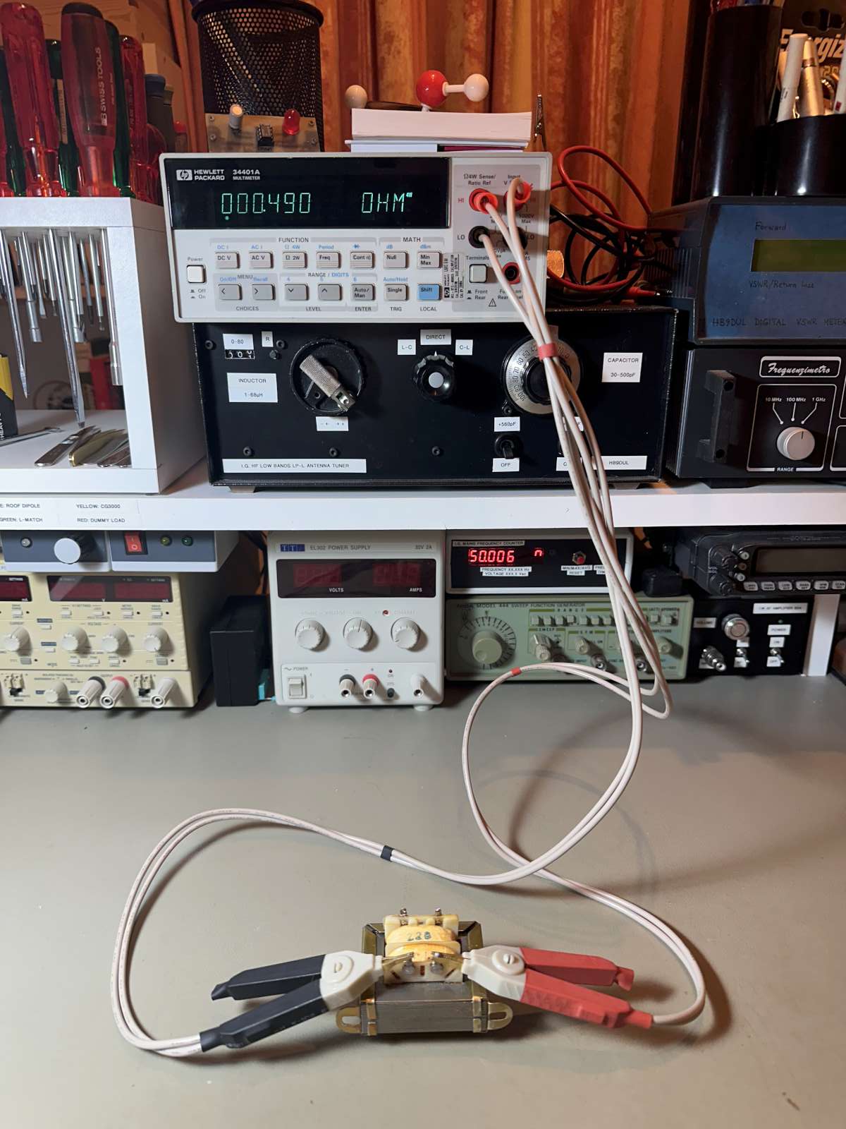
Measuring Rs with the 4-wire method.
(click to enlarge)
The inter-winding capacitance Cps can also be directly measured with a capacitance meter and is 25.3pF in this case. Here again the Agilent U1732C was used as it allows measuring such a small capacitance at 100Hz and not at high frequency.
For the core losses resistance Rc, we need to measure the losses in the core. This will be described later on when we use the power analyzer to measure the power drawn by the transformer when it's idling without load. We will find that at 238.0V the transformer absorbs 1.64W and we calculate:

Significant effort was put into finding resonances due to Cp and Cs, but none was found while sweeping from 1Hz to 2MHz, especially when shorting the other winding to measure only Cp or Cs. I have to figure out a better method for this, but I'll leave these to another time.
So, we managed to find Lp, Ls, Lh, Rp, Rs, Rc and Cps. And we already know ü. Let's summarize:
| Magnetizing inductance | Lh = 12.559H |
| Primary leakage inductance | Lp = 3.670H |
| Secondary leakage inductance | Ls = 18.19mH |
| Core losses resistance | Rc = 34.54kΩ |
| Primary resistance | Rp = 194.87Ω |
| Secondary resistance | Rs = 0.490Ω |
| Primary to secondary capacitance | Cps = 25.3pF |
| Primary capacitance | Another time |
| Secondary capacitance | Another time |
| Transformer ratio | ü = 20.1 |
We couldn't find all the parameters, but most of them are there. Because of the saturation, they are not accurate, but at least we now know how to measure them.
By knowing the geometry of the core and the number of turns, we can also try to estimate the primary and secondary inductances Lpo and Lso. If the (relative) magnetic permeability μr of the core is high (which is the case of an iron core) and there are no (or very short) air gaps in the loop, we can assume that all the magnetic flux is uniform and completely flows inside the core. The corners of the core are approximated by considering only the distances along the axis and ignoring how the field really bends.
We can draw an approximated equivalent circuit where a magnetic potential θ is generated by the current in each winding and a magnetic flux Φ flows into a loop made of reluctances Rm. Reluctance is the equivalent of resistance in a magnetic world, some sort of "magnetic resistance".
The reluctance of a straight section of core of length ℓ and of constant cross-section S is calculated with the formula:

For sake of completeness, the permeance Λ (capital "lambda") is the inverse of the reluctance Rm. The permeance is measured in Henrys and the reluctance in H−1, of course.

The permeability of vacuum μ0 is a well-known constant and is equal to 4π·10−7H/m. The relative permeability of the iron core μr is a different story: it depends on the material and its saturation. It's often in the several hundred range, usually less than one thousand. By tweaking its value, it was found that a value of 900 gives surprisingly good results that match the inductances measured before. This is cheating, somehow, but without knowing the value of μr, I would have probably chosen something between 700 and 1'000 as iron usually is in this range.
The transformer core has been divided in several segments each modeled with a reluctance by taking their respective length ℓ and cross-section S as summarized in the drawing below:
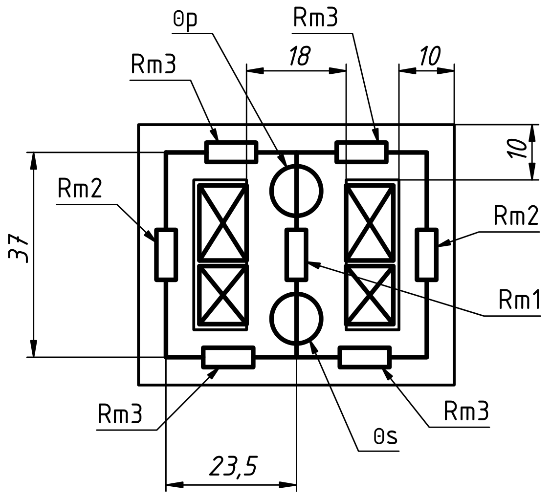
Equivalent magnetic circuit of our transformer.
Each branch is represented by a reluctance Rm and each
winding by a magnetic potential (magneto-motive force) source
Θ. (click to enlarge)
Reluctance Rm4 is not drawn here because it was an afterthought. It models the mounting holes in the edges where the cross section of the core is reduced for 3mm or so. Finally, their effect is quite small on the total reluctance.
| ℓ1 = 37mm | S1 = 324mm2 | Rm1 =117'000H−1 |
| ℓ2 = 23.5mm | S2 = 180mm2 | Rm2 =133'000H−1 |
| ℓ3 = 37mm | S3 = 180mm2 | Rm3 =210'000H−1 |
| ℓ4 = 3mm | S4 = 90mm2 | Rm4 =34'000H−1 |
| ℓtot = 121mm | Rmh =389'000H−1 |
The total reluctance Rmh is obtained by calculating the equivalent circuit:

Unfortunately, this method only allows determining the main flux Φh. Leakage flux Φσ cannot be calculated because we supposed that all the flux is inside the core for calculating our reluctances, therefore only the primary and secondary winding inductances Lpo and Lso can be calculated with this method. The mutual inductance and the coupling factor cannot be determined without knowing the leakage flux. This could be done with a magnetic field simulation software, but I don't have one on hand and I'll leave this for another time.
Still, with this simple model when the reluctance is known, inductances can then be calculated with the equation:

By using Np = 2'200 we find Lpo = 16.451H and with Ns = 109 we get Lso = 45.06mH that are good approximations of what has been measured before. As described before, the unknown value of μr was tweaked to fine tune the results and is probably a bit cheating but the goal here is only to explore the method.
A regular linear power supply mains transformer is not supposed to saturate, at least in theory. Usually, the primary winding has enough turns to make sure that the magnetic flux in the core is kept below saturation. Saturation degrades transformer performance by increasing losses in the core and by reducing the coupling factor.
So, to measure the saturation of a core that is not supposed to saturate, one can increase the voltage or reduce the frequency. A higher voltage is risky and easily leads to insulation problems that can irreversibly damage the transformer (don't ask me how I know it...). Therefore, the first saturation measurement was done at 1Hz instead of 50Hz. This was quite a complicated setup that turned out to be unnecessary as this particular transformer indeed saturates at 230V and 50Hz. It actually begins saturating around 64V. So, the measurement at 1Hz was a waste of time. This was quite a surprise but explains why losses are high.
We want to measure and display the magnetizing curve of the core, i.e. the magnetic induction B as a function of the magnetic field H. As a reminder, the magnetic field H is measured in A/m and is independent of the material. The magnetic induction B, on the other hand, is measured in Teslas and is defined as:

The magnetic flux Φ is the magnetic induction in a surface area and is measured in Wb or in T·m2. As a sidenote, depending on where in the world you learned electromagnetism, you may be used to slightly different definitions of B and H.
When current flows through a winding, it generates a magnetic field which is directly proportional to it. Here, we choose to drive a current in the primary winding, but any winding will do. By measuring the current in this winding, we can calculate the magnetic field in the core with the following formula:

Where i(t) is the instantaneous current as a function of time and ℓp is the length of coil, that in our case is 12.5mm.
The current i(t) is inferred by probing with an oscilloscope the voltage drop on a 1kΩ resistor in series with the winding as illustrated in the figure below.
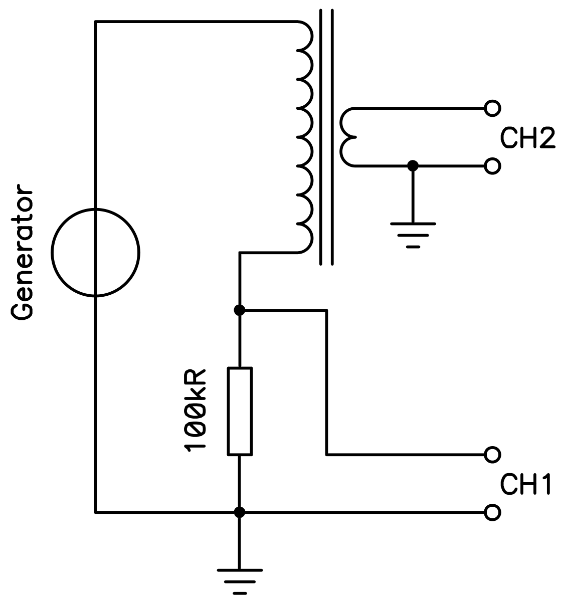
Setup for measuring the saturation of the core.
(click to enlarge)
Getting the magnetic induction is a bit trickier: we cannot measure the induction directly with a magnetometer mainly because I don't have one, but also because this would require cutting the core open and ruin its geometry. But there is another way: we can measure the induced voltage and use some math. In fact, the derivative of the magnetic induction is proportional to the induced voltage as describe by:

Therefore:

Here, we decided to use the secondary winding to measure us(t) simply by connecting the other probe of oscilloscope. In theory, one could use the same winding used to set the current, but then he should compensate for the voltage drop caused by the current in the winding resistance. When available it's much simpler to use a different winding.
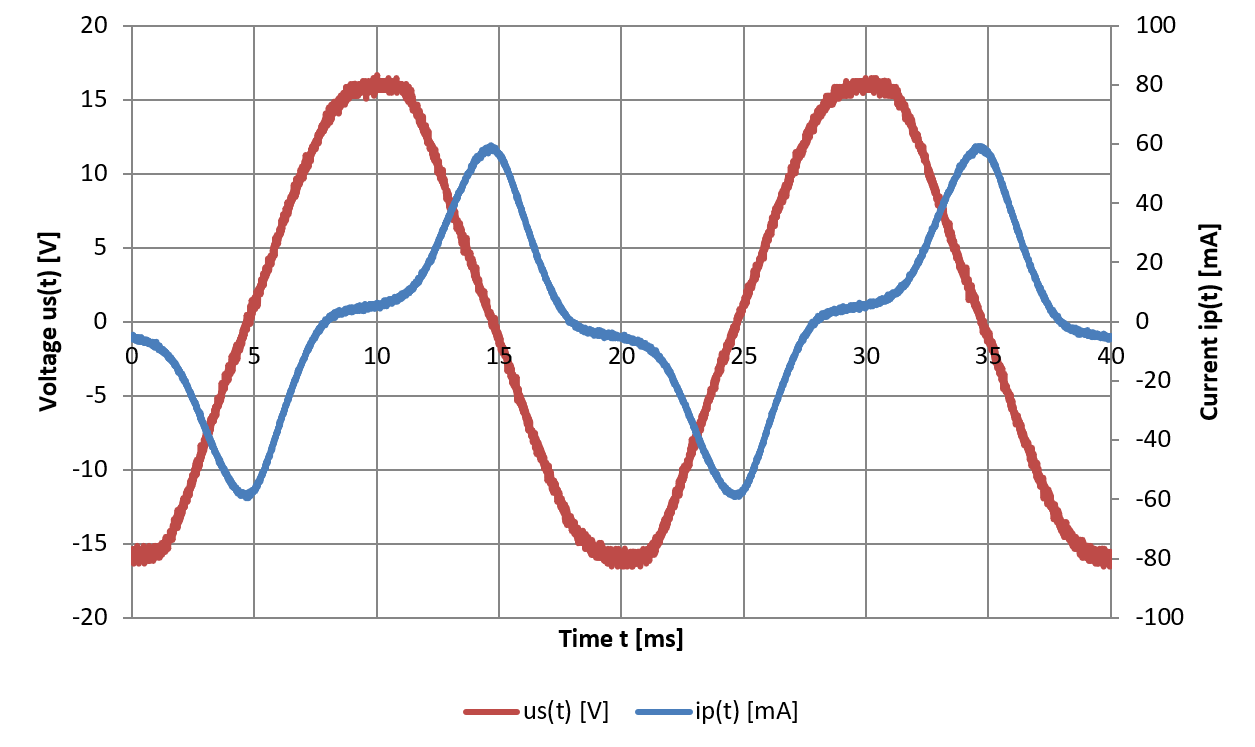
Secondary voltage and primary current as measured by the oscilloscope.
The current has simply been converted from the voltage drop across the
resistor. (click to enlarge)
We are now one integral away from the magnetic induction B. Unfortunately, my oscilloscope cannot do integrations with its own math functions, but data can be exported and easily integrated in a spreadsheet application.
Before integrating, it's important to remove any DC offset in the measurements. All oscilloscopes introduce a tiny DC offset, maybe just a few millivolts, but enough to slant the integral up or down. This is not a big deal; one must simply subtract an offset so that the integrated curve stays horizontal.
After the integral is calculated, another offset compensation must take place. This time it's because the measurements don't start exactly at the beginning of an AC cycle where the integrator is supposed to start at zero. Another way of doing this would be to delete the data of the partial cycle at the beginning or to accurately adjust the trigger of the oscilloscope to start precisely at a zero crossing. I chose to compensate for the offset because it's easier to do.
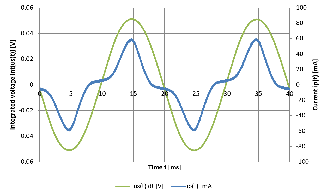
After integrating the secondary voltage we obtain these curves (the
current is still the same as before). (click to enlarge)
A first look at the signals as measured by the oscilloscope: although the voltage provided by the generator (or variac) is indeed sinusoidal, the current in the primary winding is "spiky". As the current increases, the saturation increases, the inductance decreases and the current increases even more. When spiky currents appear on an inductor driven with a sinusoidal voltage, saturation is the first suspect.
After integration, we can plot B(H) and see the magnetizing curve of the transformer. We can also clearly see the hysteresis curve of the core, i.e. the graph is a "loop" that has a path for increasing H and another one for decreasing H. By the way, the loop turns in a counterclockwise direction.
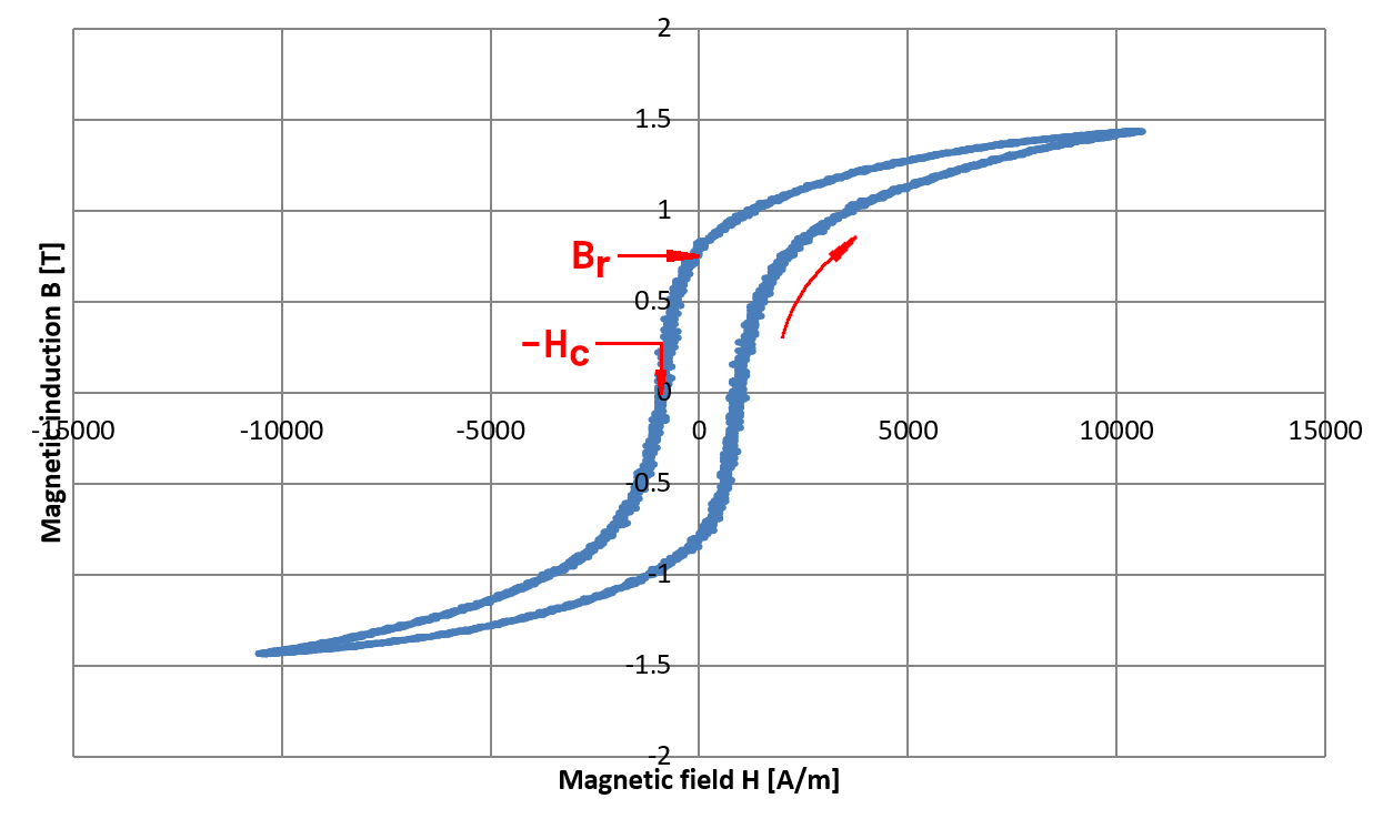
B(H) plot of the core.
The same curves have simply been scaled to A/m and T and plotted as a
function of each other.
The coercive force Hc and the remanence induction
Br have been highlighted. (click to enlarge)
While we are at it, we can also see the coercive force (or coercive field) Hc and the remanence induction (or remanent magnetization or residual magnetism) Br. The steel core acts as a magnet: when the magnetic field H returns to zero, the magnetic induction B diminishes along the hysteresis curve, but does not drop to zero and the core stays magnetized. The magnetic remanence Br is the magnetic induction that is left in the core after the magnetic field H has been removed. A good transformer core has a narrow hysteresis curve and a low Br, a good magnet material has a wide curve and a high Br. The coercive force Hc is the magnetic field that is required to zero the remanence and bring the induction back to zero. Here we have Br = 0.692T and Hc = 882A/m.
The permeability μ of the core is simply the slope of the curve. This depends on the magnetic field and on the hysteresis. The relative permeability μr is given by:

Usually, μr is measured when the core is not magnetized: where B(H) = 0 i.e., where it crosses the horizontal axis. We can calculate that μr is 847. We can double check our measurements by determining μr when H is very high and the iron has saturated: we should get 1 but we find 8.5. This result is not as bad as it may seem: 8.5 is of course quite greater than 1, but we can still consider that the core is not fully saturated yet. And 847 is not only a very plausible value for an iron core, but also not that far from the 900 that we tweaked in our inductance calculation. Considering that we are unsure of the exact number of turns and that the exact magnetic length of the coil is very difficult to estimate, we can be quite happy of this result.
We know that this transformer was designed to work at 50Hz. But can it be used to transform audio signals too? What is its bandwidth? We know that it saturates, and we have seen when measuring the saturation of the core that the signal is distorted, but this only happens when the voltage is too high, or the frequency is too low. We also found that at 50Hz saturation starts at 64V. Let's use a voltage low enough and see how the transformer behaves at different frequencies.
The primary is connected to a function generator and the output is adjusted for a sine wave of about 10VRMS. This is low enough to prevent saturation at 50Hz and probably a bit below but is high enough to still be able to measure something reliably on the secondary that is ü = 20.1 times smaller. The secondary is left &open;open&opne; and is "only connected" to the scope probe.
If the transformer was perfect, we would expect a flat response at all frequencies. The line should be at a height of 1/ü = 0.0498 corresponding to −26.1dB. In practice, this is what it was measured:
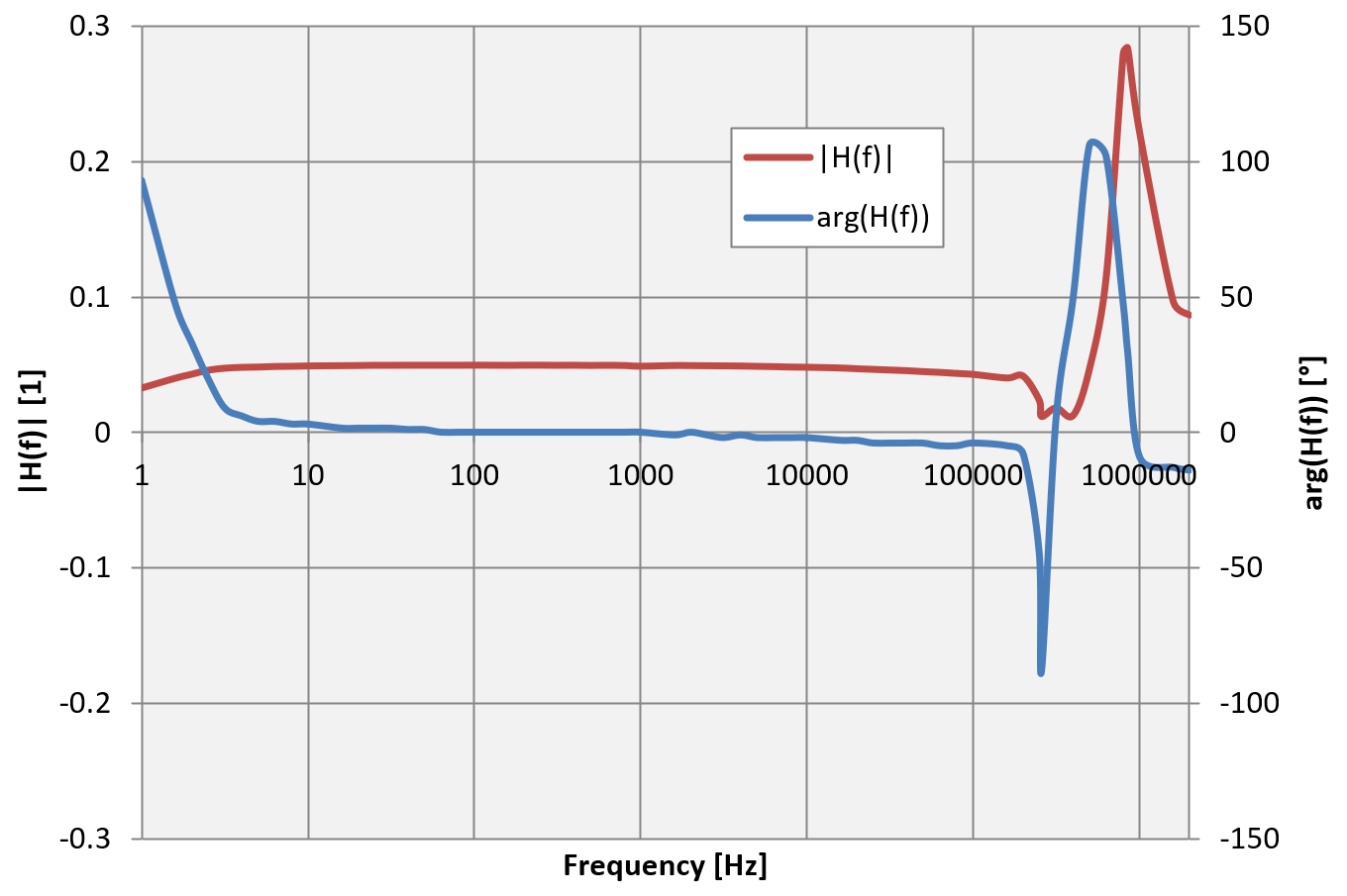
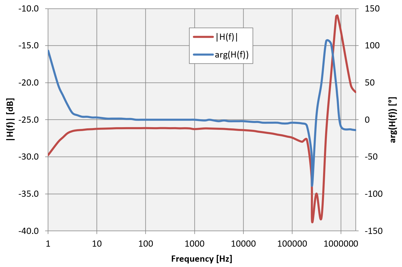
Transformer frequency response, both linear (left) and in dB (right).
(click to enlarge)
We see that the response from 2Hz to 200kHz is pretty flat and around 0.5 or −26dB. We clearly see resonances, especially one (or two) series resonance(s) around 315kHz and a parallel resonance around 1MHz. These are due to the winding capacitances.
For very low frequencies saturation kicks in and ruins the response. This can be seen in the following two measurements: the 1Hz sine wave is heavily distorted and is spiky, while the 3.18Hz one is almost perfectly sinusoidal.
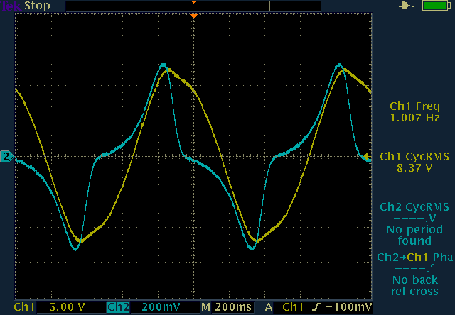
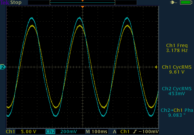
At low frequency core saturation distorts the signal; at 1Hz
saturation is significant (left), at 3.18Hz the signal is almost sinusoidal
(right). (click to enlarge)
This is even more apparent if we switch to a square wave: at 1Hz we clearly see that the signal is "short circuited" as soon as the core saturates. But already at 10Hz the square wave is almost undistorted.
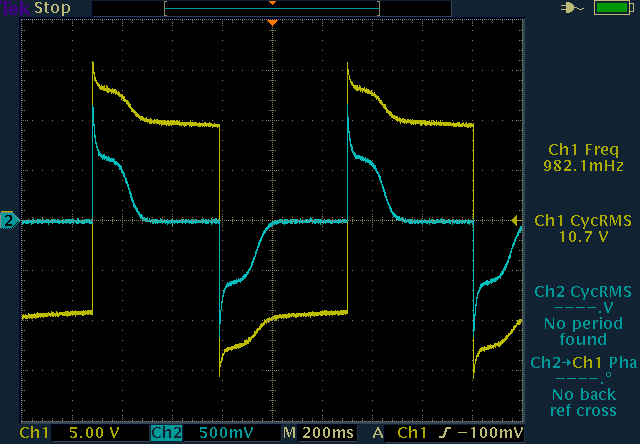
Transfer of a square wave: at 1Hz (and 10V) saturation is significant
(left), but already at 10Hz the signal goes through almost undistorted
(right). (click to enlarge)
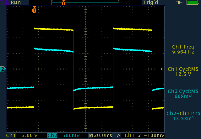
By increasing the frequency, we see that the transformer transfers the wave even better and with lower distortion. At 100Hz the transformer works beautifully. But because square waves have a high harmonic content, at higher frequencies the highest harmonics start to tickle the resonances of the transformer and ringing appears.
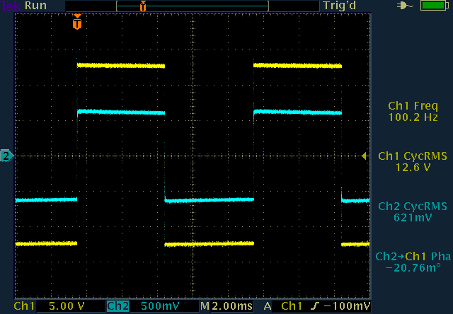
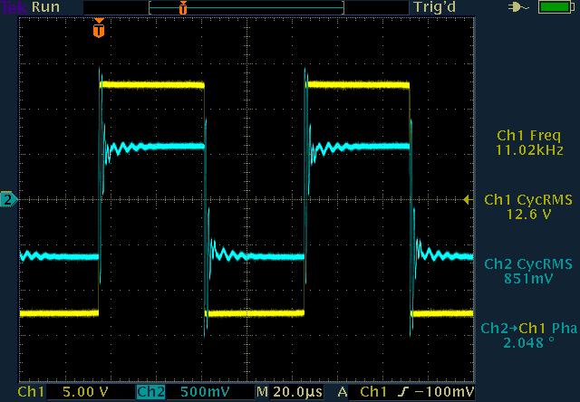
At 100Hz the square wave is transferred without distortion (left), but
when the highest harmonics start tickling the resonances of the transformer
ringing appears, here at 11kHz (right). (click to enlarge)
A triangular wave was also measured. As with the square wave, at 10V amplitude it's nicely transferred between 10Hz and 10kHz:
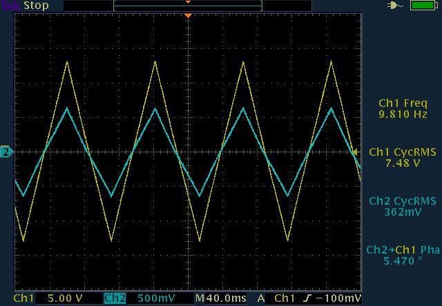
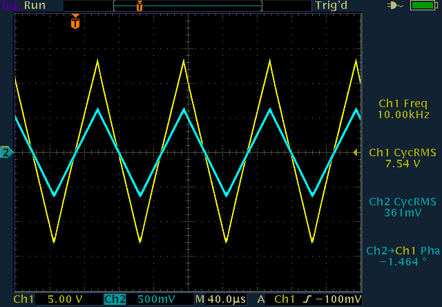
Transfer of a triangular wave at 10Hz (left) and 10kHz
(right). (click to enlarge)
It should also be noted that there is no phase shift between the primary and secondary: the signals are in phase. This is how an ideal transformer is supposed to behave.
In summary, this transformer is not designed to transfer audio signals, it doesn't have an ultra-flat response or a particularly wide bandwidth suitable for a HiFi application, but it surely transfers audio frequencies in a reasonable way.
Ok, let's now connect the transformer to a power analyzer and determine some of its AC characteristics when used as a mains transformer. First, we power up the power analyzer and let it warm up for about one hour. Then we take a reading with no load connected to it: we measure 238.1V, 0.7mA and 0.06W: this gives an idea of the precision of the instrument and the smallest values that can be measured with it. On the other end of the scale this Valhalla Scientific 2100 Power Analyzer can measure 20A and 600V for a maximum of 12kVA. Our transformer is only rated 15VA, therefore we are a bit on the low side of what the analyzer can do, but the measurements will still be useful.
Let's now connect the primary of the transformer and see what happens: we measure Up = 238.0V, Ip = 34.8mA and Pp 1.64W. The secondary is left open, but its voltage is measured at Us = 11.73V. The transformer is dissipating 1.64W, mainly in saturating its core. This is because the primary current in the primary winding is only 34.8mA and the ohmic losses are just 0.24W: the remaining 1.40W is lost in the core. We can also calculate that the apparent power is Sp, the power factor is cos(φp) and phase angle φp.


It's not a surprise that our idle transformer (with no load) behaves as a large inductor.
We can now calculate the magnitude of the primary impedance:

The resistive part of that impedance is just:

And the reactive part can be found with:

If we want, we can also express the impedance in its complex form:

From the reactance we can also determine inductance:

This is more than what we have measured before directly with the inductance meter. Now, the accuracy of my power analyzer is not great because we are measuring small values for its range and because it was last calibrated in the '80s... but again, the goal is to explore how measurements are done and not the actual values.
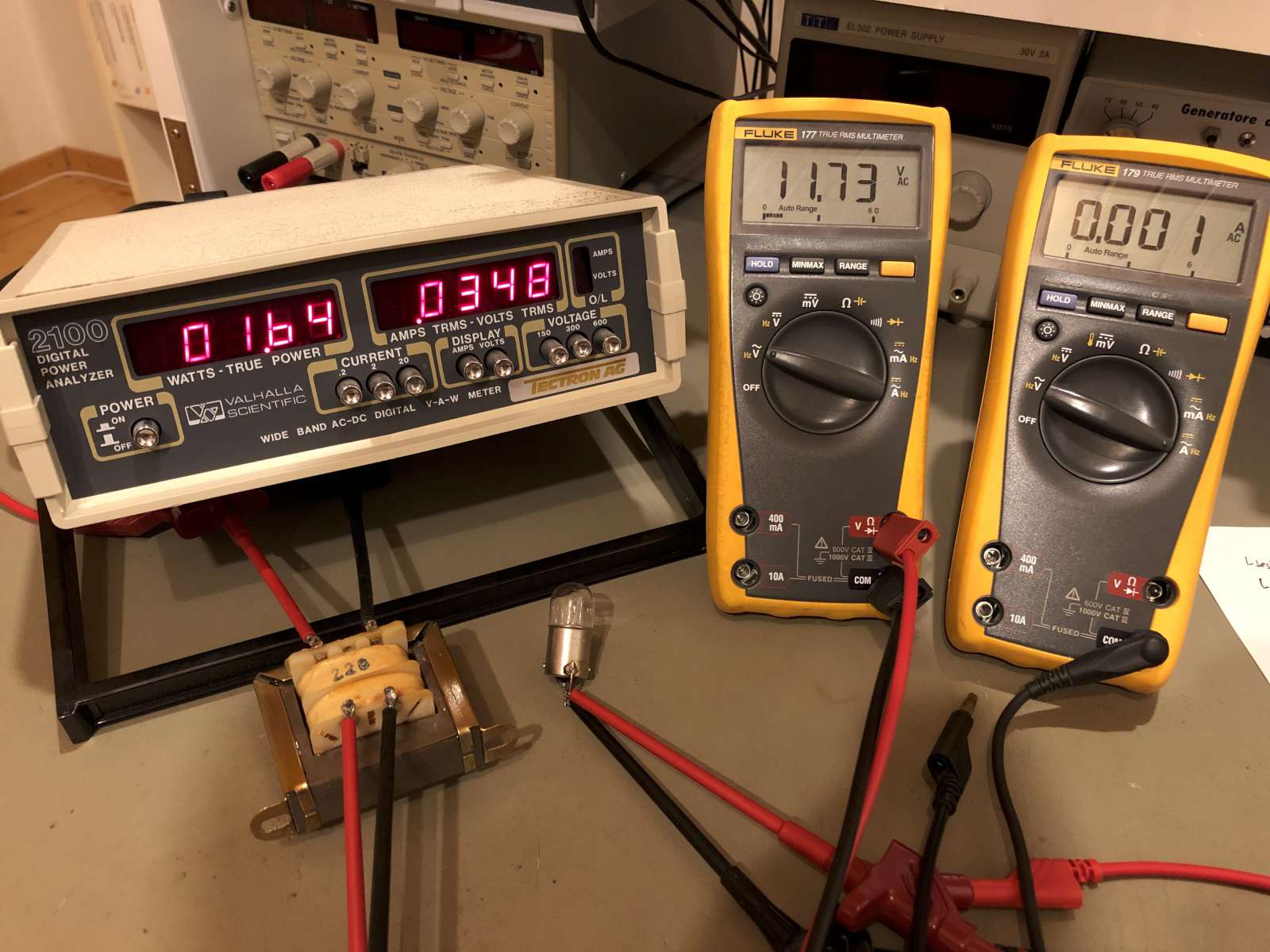
Measuring the power of the transformer when idle (the light bulb is
not connected).
The power analyzer measures the primary side while the two multimeters
measure the secondary side. (click to enlarge)
If we connect a 12V 5W (car) lightbulb on the secondary, we start drawing some active power. On the secondary side, the voltage drops to 11.36V and the current is 360mA. The power absorbed by the lightbulb is:

This power is active as the lightbulb is a resistive load, so the apparent power is also Ss = 4.08VA and there is no reactive power Qs = 0var.
On the primary side we now have Up = 238.1V, Ip = 40.2mA and Pp = 5.74W. Ohmic losses are 0.32W on the primary and 0.06W on the secondary. Calculating the power budget, we find that the losses in the core are 1.28W, roughly unchanged. This is also not a surprise as saturation losses don't depend on the load. The apparent power is now 9.57W, cos(φ) = 0.599 and the phase angle is 53.1°: because of the increased active power the transformer seen from the primary behaves less as an inductor and more as a resistor.
Doing the same math again, we find that the primary impedance is now (3'552+j4'740)Ω and we can determine the inductance of the reactive part being 15.1H. The inductance should not have changed (the number of turns and the voltage are still the same) but we see that its value is now closer to the expected 16.229H. This confirms that the measurements of this power analyzer are not accurate for small loads.
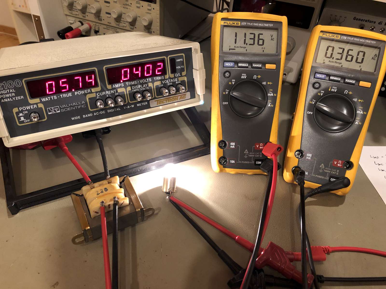
Measuring the power of the transformer when loaded with a 5W light
bulb.
The power analyzer measures the primary side while the two multimeters
measure the secondary side. (click to enlarge)
Finally, I tried to connect a capacitor as a load to see what happens. I connected two 470μF electrolytic capacitors back-to-back and obtained a 235μF non-polarized capacitor. This value was actually measured and by chance it happened to be exactly 235μF, i.e. exactly one half of 470μF. The equivalent series resistance was also measured at 0.19Ω with an ESR meter.
With the capacitor, the voltage on the secondary side is now 12.03V, the current is 856mA, the apparent (and reactive) power is 10.3VA (10.3var) while the actual active power is only 0.14W. The power factor is 0.01 and the phase angle is 89.2°, as expected for a good capacitor. On the primary side, we measured 238.9V, 21.5mA and 2.69W. Now we have ohmic losses in both the primary and the secondary of 0.09W and 0.37W. Calculating the power budget again, we find that the losses in the core are 2.09W, roughly unchanged. The apparent power is now 5.14W, cos(φ) = 0.524 and the phase angle is −58.4°: because of the large capacitive load the transformer as seen from the primary side stops behaving as an inductor and looks like a capacitor. The impedance of the primary is now (5'819−j9'466)Ω and we can determine the capacitance of the reactive part being 336nF.
Actually, these measurements don't tell if the load is inductive or capacitive: the power analyzer gives the active power and multiplying voltage and current gives the apparent one, but if cos(φ) is lower than 1, it could be either capacitive or inductive. But there is an easy trick to tell them apart: connecting a capacitor in parallel and see what happens. I used 100nF, that I chose smaller than the expected 336nF. By connecting it in parallel with the transformer primary I observed the primary current increasing, confirming that the impedance is indeed capacitive: connecting a capacitor in parallel to another capacitor increases the total capacitance, makes the load more capacitive and both the current and the reactive power increase. Should the impedance have been inductive, adding an extra capacitor would have partially compensated the inductive load and both the reactive power and the current would have decreased.
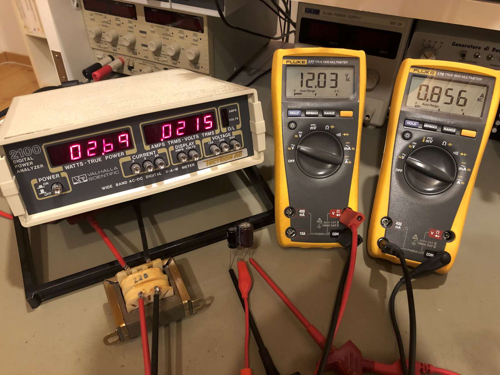
Measuring the power of the transformer when loaded with a 235μF
capacitor.
The power analyzer measures the primary side while the two multimeters
measure the secondary side. (click to enlarge)
What at the beginning looked like a simple rainy Sunday afternoon project ended up being quite a technical challenge that occupied many days of work. Several aspects of a simple transformer could be investigated. Some others deserve to be revisited because the results do not perfectly match, like the voltage ratio derived from inductance measurements or the transformer resonances that could not be found. I definitely learned that power transformers can be designed with some saturation to save cost and materials while still working reasonably ok. The more time I spend playing with this transformer the more I have the feeling that I only scratched the surface. How would a ferrite core transformer behave? And what about a transformer with a leaky core like a flyback transformer? And a transformer designed to saturate like a ferro-resonant one? A lot of interesting questions but lacking more rainy Sundays they'll have to wait.
| [1] | See Nuova Elettronica, Vol. 6, p134. The denominator has been changed from 14'000mm4/VA to 15'500mm4/VA to account for 5% of space in the core that is occupied by the insulating varnish on the steel sheets. |
| Home | Electronics | Page hits: 009172 | Created: 01.2024 | Last update: 01.2024 |