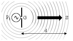
When a transmitter is connected to an antenna and radiates power, it's often interesting to know what is the electromagnetic field strength at a given distance. The following diagram summarizes the problem:
A transmitter of power Pt is connected to an antenna of gain G that radiates in the surrounding space. We are interested to know the intensity of the field S, E and H at the distance d from the transmitting antenna.
This measurement must be done in the far field region, otherwise the formula used here are not valid. This means that the measurement must be taken at an adequate minimum distance from the transmitting antenna, so that we can neglect its shape and suppose that we have a nice and spherical wave. This calculator is not intended for near field analysis.
The power provided by the transmitter is radiated by the antenna. As the waves leave the antenna, they spread on the surface of spheres of increasing radius as they travel away. In a very similar way, when dropping a stone in a pond, circular ripples leave the point of impact and become larger and larger in diameter as they travel away.
Wave-fronts can be approximated with spheres only if we are far enough from the antenna that originated them, so that its shape can be neglected and considered a point source. For this reason, we can only consider the far field region.
As the spheres become bigger and bigger, their surface increases with the square of the distance d2. The total amount of power carried by the wave doesn't change (without losses), so the same power spreads on a larger and larger surface, explaining the 1/d2 dependence of the power density of the wave and finally of the received power.
Furthermore, this simple model doesn't take into account any effect of the ground: the transmitting antenna needs to radiate in free space and to have line of sight with the measuring point. Antennas that use the ground as part of them, like vertical monopoles, cannot be calculated reliably. Ground can also reflect waves and reflections are not take into account, only the straight path is considered. The effect of the ground is less important at microwave frequencies, since it tends to absorb energy instead of reflecting it back and since the distance to the ground in terms of wavelength is much larger. In other words, in most cases, the model is ok for wavelengths shorter than a few meters, say frequencies from the VHF band and up.
This being said, with our simple spherical waves model, calculating the power density at a given distance d is quite straightforward and depends mainly on the geometrical considerations above, as stated by the following equation:

Here, we include the antenna gain g, which is a measure of the ability of the antenna to concentrate (direct) the power in a given direction (directivity). The antenna gain also includes the losses of the antenna, and here, for simplicity, we also include any additional loss of cables or devices that are between the transmitter and the antenna.
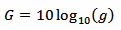
Here we need the gain g in terms of power ratio, so the usual gain G in dB must be converted first with:
Now, the strength of an electromagnetic wave can be expressed in terms of electric field strength E (measured in V/m), of magnetic field strength H (measured in A/m) or of power density S (measured in W/m2).
E, H and S are actually vectors and S is also called Poynting vector. Here, since we are in the far field region, E and H are at 90° and in phase to each other, so that we can consider only the magnitude and neglect the vectors. S, as a vector, is oriented in the same direction of the propagation while E and H are orthogonal to it (transverse wave) as summarized in the diagram below:
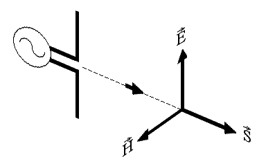
The direction of the electric field E also defines the polarization of the wave.
It's very common to describe the intensity of an electromagnetic field in terms of the electric field strength E rather than H or S, but in the far field region, they are all equivalent and related by the following two equations:
 and
and
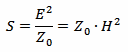
Where Z0 is the characteristic impedance of vacuum that is Z0 = 120π Ω ≈ 377 Ω
So, we can easily convert S into E and H.
While we are at it, we can also calculate the effective isotropic radiated power (EIRP), given by the following equation:

It's is just the transmitter power Pt multiplied by the antenna gain g. PEIRP can easily be a fairly large number. But it's not a "true"quot; power: antennas do not amplify power, they just concentrate (direct) it in a given direction. The total radiated power is still Pt, but in the direction of the gain of the antenna (and in this direction only) the antenna behaves as an isotropic antenna fed with PEIRP. An isotropic antenna is an antenna that radiates uniformly in all directions; in other words it's an antenna that is not directive at all.
Please remark that these assumptions and equations are only valid if all the following conditions are met:
To use this calculator, enter the antenna gain G, the receiver distance d and one of the other values. Then click the "calculate" button next to it to compute all the other values.
You can also use this calculator to convert only between E, H and S: in this case, just enter any valid value for G and d.
Let's take an example: in the picture below we can see a GSM base station about 100 m away from the wooden pole on the left.

Assuming that the transmitter has an output power of Pt = 20 W, that the cable has a loss of 3 dB, and that the antenna has a gain of 18 dBi, we can estimate the field strength at 100 m distance. To take into account the loss in the cable, we just have to deduce the 3 dB loss from the 18 dBi gain and use a modified antenna gain of G = 15 dBi.
In one click we find the electrical field strength E = 1.4 V/m, the magnetic field strength H = 3.7 mA/m and the power density S = 5.0 mW/m2. We also find the effective isotropic radiated power PEIRP = 633 W.
This assumes that the antenna is aiming in this direction blasting all the power towards the wooden pole of the picture. In reality, the antenna is probably oriented a little higher, so that the majority of the energy flows overhead and reaches a larger distance. So a real measurement will probably show a slightly lower field.
| [1] | C.-A. Balanis. Antenna theory, analysis and design. Wiley, 1997, Chapter 2. |
| [2] | P.-G. Fontolliet. Traité d'Électricité, Vol. XVIII: Systèmes de télécommunications. Presses Polytechniques et Universitaires Romandes, 1996, Section 3.9. |
| [3] | The ARRL Antenna Book, 19th edition. American Radio Relay League, 2000, Page 17-11. |
| [4] | X. Lagrange, P. Godlewski, S. Tabbane. Réseaux GSM-DCS. 4ème édition. Hermes Science Publications, 1999, Section 6.2.1.2. |
| Home | Electronics | Index | Page hits: 185868 | Created: 09.2000 | Last update: 11.2012 |