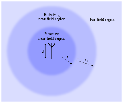
Diagram showing and antenna surrounded by its three field regions.
When a high frequency current flows in an antenna, it generates a high frequency electromagnetic field in the surrounding space. The detailed structure of this field is usually quite complex and strongly depends on the antenna shape. Close to the antenna, except in some simple academic cases, there is very little we can say about the electric and magnetic fields without involving complex numerical calculations. But the good news is that, as we move away from the antenna, the field tends to look like spherical waves. And the greater the distance, the better the resemblance with spherical waves. Spherical waves are very handy because many calculations can be performed with simple equations.
Diagram showing and antenna surrounded by its three field
regions.
So, as shown in the above diagram, the surrounding space of an antenna is usually subdivided (classified) into three regions: the reactive near-field region, the radiating near-field (Fresnell) region and the far-field (Fraunhofer) region. These regions are useful to identify the field structure to know which simplification can be applied, but there is no precise boundary nor abrupt change in the field configuration.
It's a region immediately surrounding the antenna where the reactive field predominates. The electric and magnetic fields are not necessarily in phase to each other and the angular field distribution is highly dependent upon the distance and direction from the antenna. Here, only numerical methods (or a lot of calculus) can determine the structure of the field. Not all this field radiates; I imagine this region like a volume the antenna needs to "prepare" the field that will actually radiate.
It's a region surrounding the reactive near-field region described above. Here, the radiation fields predominates, the electric and magnetic fields are in phase, but the angular field distribution is still dependent upon the distance from the antenna. This means that almost all the field in this region radiates, but since we are still close, the contribution of the different parts of the antenna make a complex field structure. In other words, we are still too close to the antenna to ignore its shape. Even if the field structure is simpler, it still requires numerical methods (or a lot of calculus) to determine the exact structure.
It's a region surrounding the reactive and radiating near-field regions described above. It extends to infinity and represents the vast majority of the space the wave usually travels. Here, all the field radiates, the angular field distribution is essentially independent of the distance from the antenna and can be approximated with spherical wave-fronts. Since we are very far from the antenna, its size and shape are not important anymore and we can approximate it as a point source. The electric and magnetic fields are in phase, perpendicular to each other and perpendicular also to the direction of propagation. This greatly simplifies the math and allows using simple calculators like the ones presented in these pages.
The reactive near-field region radius r1 is determined by the following equation:
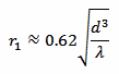
Where d is the maximum dimension of the antenna and λ is the wavelength.
The radiating near-field region radius r2 is defined by the following equation:

Of course, λ can be found with:

Where f is the frequency and c0 is the speed of light, c0 = 299'792'458 m/s.
The radii r1 and r2 are not exactly radii of spheres (they can be much smaller than the d), but have to be interpreted as distances from the closest antenna point defining some sort of envelope around the antenna itself.
For very small antennas (d < 0.096 λ), r1 is larger than r2, meaning that there is no radiating near-field region.
Enter the frequency f, the dimension d, and click the "Calculate" button to compute the two radii r1 and r2.
Let's have a look at a few examples: the picture below shows a ground plane antenna designed for a frequency f of 2'450 MHz and its maximum dimension d is 5.4 cm (from the top of the middle rod to the tip of one of the fins).
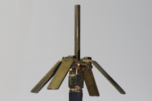
With this calculator we find the reactive near-field region being 2.2 cm and the radiating near-field region being 4.8 cm.
The helical antenna in the picture below still works at 2'450 MHz, but is much bigger: the largest dimension is 43 cm.
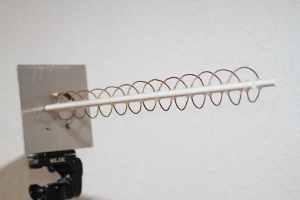
This time we find the reactive near-field extending up to 50 cm and the radiating near-field up to 3.0 m. All the rest of the space is, of course, the far field.
In this last picture, one can see a tower working as a vertical monopole. The tower is 126 m high and works at 765 kHz. Vertical monopoles use the ground as a mirror and are actually only the half of the antenna, the other half is "reflected" in the ground. Therefore, here we have to use a dimension d twice as the height of the tower, so d = 252 m.
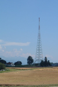
So, we find a reactive near-field extending to 125 m and a radiating-near field extending to 324 m.
| [1] | C.-A. Balanis. Antenna theory, analysis and design. Wiley, 1997, Chapter 2. |
| Home | Electronics | Index | Page hits: 115012 | Created: 09.2000 | Last update: 11.2012 |