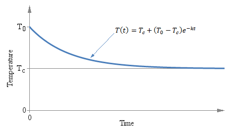
Temperature T as a function of time t of a thermometer initially at temperature T0 immerged in a liquid at temperature Tc at time t = 0.
The exponential decay is a very common phenomenon in physics and is found in many domains like heat transfer, fluid flow, electricity (RL or RC circuits) and many others. Often, to measure something involving an exponential decay, we wait until the decay is "over" and only once everything is steady, we take our measurement. But there is another option: three readings taken while the decay is still significant are enough to find out the final steady value without waiting.
Let's take the example of measuring the temperature of a liquid. We call Tc the temperature of the liquid and this is the value we are looking for. Now, we have a thermometer that is initially at a different temperature, T0. When we put the thermometer in the liquid, heat is transferred between the liquid and the thermometer until the latter reaches the same temperature Tc as the liquid, providing the result we want. The only problem is that this theoretically take an infinite amount of time. In other words, the amount of heat transferred between the liquid and the thermometer is proportional to the difference of the temperatures of the two. As the temperature delta decreases, the heat transfer also decreases slowing down the process.
The heat capacity of the thermometer is supposed to be much smaller compared to the one of the liquid, so that we can assume that immerging the thermometer in the liquid will not change Tc.
It doesn't matter if the initial temperature T0 is above or below Tc, the exponential behavior is the same and the curve always converges to Tc. The following graph shows the situation:
Temperature T as a function of time t of a thermometer
initially at temperature T0 immerged in a liquid at
temperature Tc at time t = 0.
This is just a classical exponential decay and obeys to a very precise low. In this case, since we are talking of heat transfer, it's the Newton's law of cooling, but equations of the same form are very common if physics. Our exponential decay function is described by the following equation:
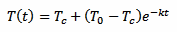
That defines the temperature of the thermometer T as a function of time t. The constant k is the time constant of the decay and defines how "fast" the curve approaches the final value Tc. The minus sign indicates that this curve always converges towards Tc as time goes by (k itself must be always positive).
The easiest and more commonly used approach to measure the temperature Tc is to put the thermometer in the liquid and wait long enough until the temperature T has settled; and the more you wait, the less the error. For example, if you wait five times the time constant k, the error will be well below 0.7%; if you wait ten times k, the error will be below 50 ppm.
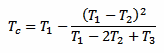
But there is another way to measure Tc without waiting a long time (and without even bothering with k). Since the exponential law is well known, it's enough to take just three measurements T1, T2 and T3 after the thermometer is in the liquid and use the following formula to immediately find out Tc:
There is only one constraint to observe: the three measurements must be taken after the same amount of time Δt. The actual value of Δt doesn't matter and it doesn't even appear in the above formula, but the time interval Δt that goes between T1 and T2, and between T2 and T3 must be the same. The following plot graphically illustrates the situation:
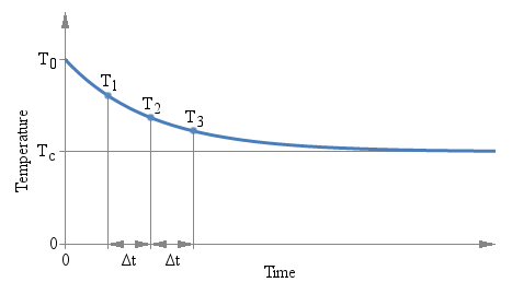
Three measurements T1, T2 and
T3 are taken after the same time interval
ΔT.
There are several interesting aspects of this method: first, you don't need to wait a long time for the value to stabilize. You can use any ΔT you want and you can find the answer while readings are still settling down. But you need to keep the accuracy of the measurement (both temperature and time) into account: a small ΔT implies a large extrapolation error.
Second, you don't need to know the time constant k of the process, which in many cases is unknown or would require additional measurements to find out.
Third, it doesn't matter which unit your instrument is measuring: temperature, voltage, current,... as long as the three values are expressed in the same unit, and that the process is controlled by an exponential decay, this method will work.
Forth, you don't need to start measuring at the precise moment when the thermometer is introduced in the liquid: T1 can be anywhere along the curve.
The following calculator will do the maths for you: just enter the three temperatures T1, T2 and T3, and hit the "calculate" button to find Tc.
Please remark that since this calculator works with any physical process involving an exponential decay (not only temperature), no unit has been specified, just use the same for all values.
We know, from the laws of physics, that our process is controlled by the following equation:
[eq. 1]
We take three measurements at time t, t+Δt and t+2Δt. We don't really care about t, that we assume equal to 0: the result will be the same. This is because here we are not looking for the initial temperature of the thermometer T0 but for the liquid temperature Tc. We can simplify our algebra by supposing that T1 is the initial temperature and still solving for Tc, avoiding an extra equation for T1. Otherwise we would have terms in e–kte–kΔt and at the end all the e–kt will cancel out. So, here we treat T1 as if it was T0, and assuming T1 is our first measurement, for T2 we have:
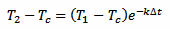 [eq. 2]
And, in a similar way, for T3 we have:
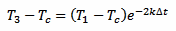 [eq. 3]
Now, taking equation 2 and squaring it we obtain:
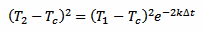 [eq. 4]
And we can also rearrange equation 3 in the following way:
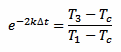 [eq. 5]
Now, putting equations 4 and 5 together, the exponential function (including the time constant k and the time difference Δt) disappears and we are left with the following equation:
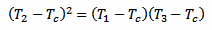 [eq. 6]
Which we can solve for Tc:
[eq. 7]
The nice thing about this equation is that all the exponentials have gone: only sums, multiplications and a division.
In the following picture, we have a cup of hot tea, a thermometer and a stopwatch. First the stopwatch is started, than the probe is put into the cup, and three consecutive readings are taken, every 4 seconds (at t1 = 6 s, t2 = 10 s and t3 = 14 s). The three readings are T1 = 45.1°C, T2 = 77.7°C and T3 = 85.2°C. With this method, we can calculate that the temperature of the tea is Tc = 87.4°C, without waiting any longer.
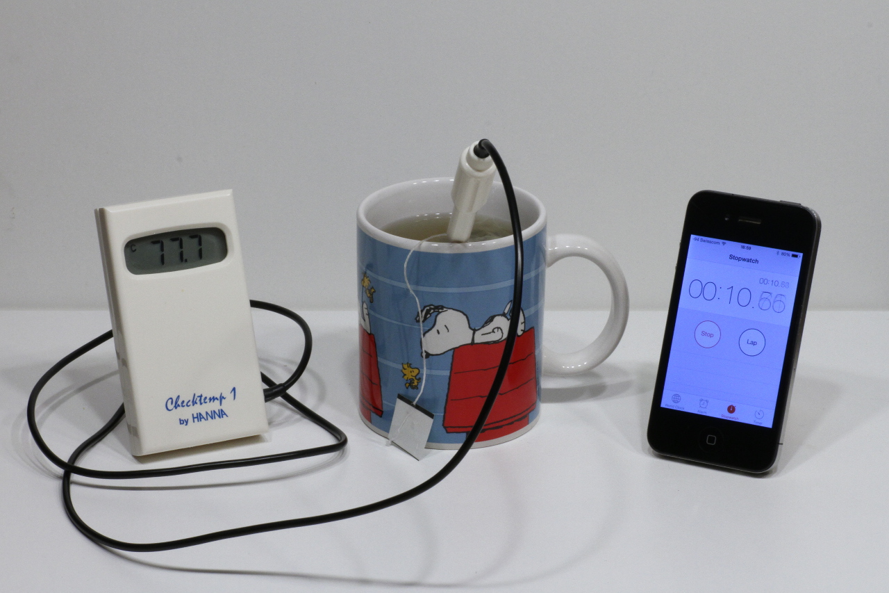
A thermometer, a stopwatch and a cup of hot tea.
Of course, this is just a simple example. Here, the time constant is quite short and waiting a few seconds more is not a problem. But if the time constant is much longer, or if the three readings can be automated and done much quicker, this method can be very handy.
An alternative method of measuring temperature has been presented. It may be useful in some situations, for example when the time constant is unacceptably long or when this algorithm is integrated in an automated system. It has the advantage of not requiring the temperature to be stable for deducing the final value. It can be used in many different domains other than thermometry, like fluid flow or electricity. But it has the drawback of requiring accurate measurements, because extrapolating a value has the effect of amplifying the errors.
| [1] | H. Matzinger. Analyse II: Cours du Prof. H. Matzinger. École Polytechniques Fédérale de Lausanne, 1994/95, Chapter X.1, pages 11-13. |
| Home | Software | Page hits: 035901 | Created: 11.2014 | Last update: 11.2014 |