
A large nuclear power plant in southern France (click to enlarge).
My interest in a Geiger counter started with the Chernobyl disaster in 1986 when I was about 10. There were a lot of discussions in the media at that time about radioactivity, dose, isotopes, the dangers of living in a radioactive area and of eating radioactive food.
You cannot see radioactivity, you can't smell it and you can't feel it neither: the only way to check if something is radioactive or not, is to use a dedicated detector. The simplest one is the Geiger counter and I definitely wanted one.
Internet was not invented yet and the only source of technical information was written on paper: books and magazines. There were several articles in the technical magazines on how to build Geiger counters but even if the circuits were quite simple, the biggest problem was to find the Geiger tube. These tubes were very rare and expensive, out of reach of a 10 years old boy. So I had to wait many years until I could buy one.
I finally bought a counter in the mid-nineties: a DIY kit sold by an Italian magazine [3]. I was not very satisfied of this instrument, because it wasn't well engineered and it wasn't very sensitive, but still it was better than nothing and quite funny to use.
Many years later, while surfing the internet, I stumbled upon some cheap Geiger tubes and decided to build my own counter, based on my own specifications with the goal of making a better instrument than the one I already had, but also to have some fun by designing a new and cool circuit.
Definitely, times have changed: it's now possible to buy tubes online for cheap and to find technical information like datasheets in just a few clicks. If only I had that back in the time I was 10...
Thinking that the problems involved in this circuit may be of some interest, I decided to share in this page a detailed description of what I did and why, so that it can be reused and modified for different tubes or working conditions. Or maybe be of some inspiration for an even better detector.
A large nuclear power plant in southern France (click to enlarge).
There is one more question: why would one want a Geiger counter? Well, it's not something that you'll use every day, but it's definitely a useful instrument. It's like a medical thermometer: you wish you'll never use it, but when you need it, it's good to have one. Nuclear power plants are part of our landscape; they are incredibly reliable, but still, a Geiger counter is worth owning, just in case...
I'm not a radiation expert or a nuclear physicist: consider this as an electronics project and not as a precise radiation measuring instrument. Also take the considerations and assumption on radiation, conversion factors and thresholds with skepticism; again, I'm not an expert.
Radioactivity is a natural phenomenon. Everything is slightly radioactive and usually there is nothing to worry about. For example, the air that we breathe contains small amount of radioactive radon; rocks and soil contain traces of radioactive elements; cosmic radiation hits the earth from deep space; and so on. On top of this natural radiation, there is also some man-made radiation that comes from the various nuclear accidents and nuclear tests that happened in the past. This is called background radiation. This means that even if no specific radioactive source or contamination is present, there is still some radiation that a Geiger counter will pick up.
Background radiation depends on location, there are some areas that are more radioactive than others; for example, because of the different composition of the nearby rocks. It also depends on the weather: when it rains, the background radiation usually rises a bit, because some slightly radioactive dust normally suspended in the air, is suddenly brought on the ground by the raindrops where it accumulates. On the other hand, snowfalls can lower the background radiation by slightly "shielding" the ground. [5]
Even the Geiger tube itself is slightly radioactive: the materials used for its construction are not perfectly inert, even if great care is taken during manufacturing to keep this radiation as low as possible. The SBM-20 datasheet reports that this particular tube has an inherent counter background of maximum 60 cpm (but the ones I have are much better than that).
When designing an instrument, one has to make some technical choices. Since I was not happy with my previous meter, I already had several ideas of features I wanted in my new one.
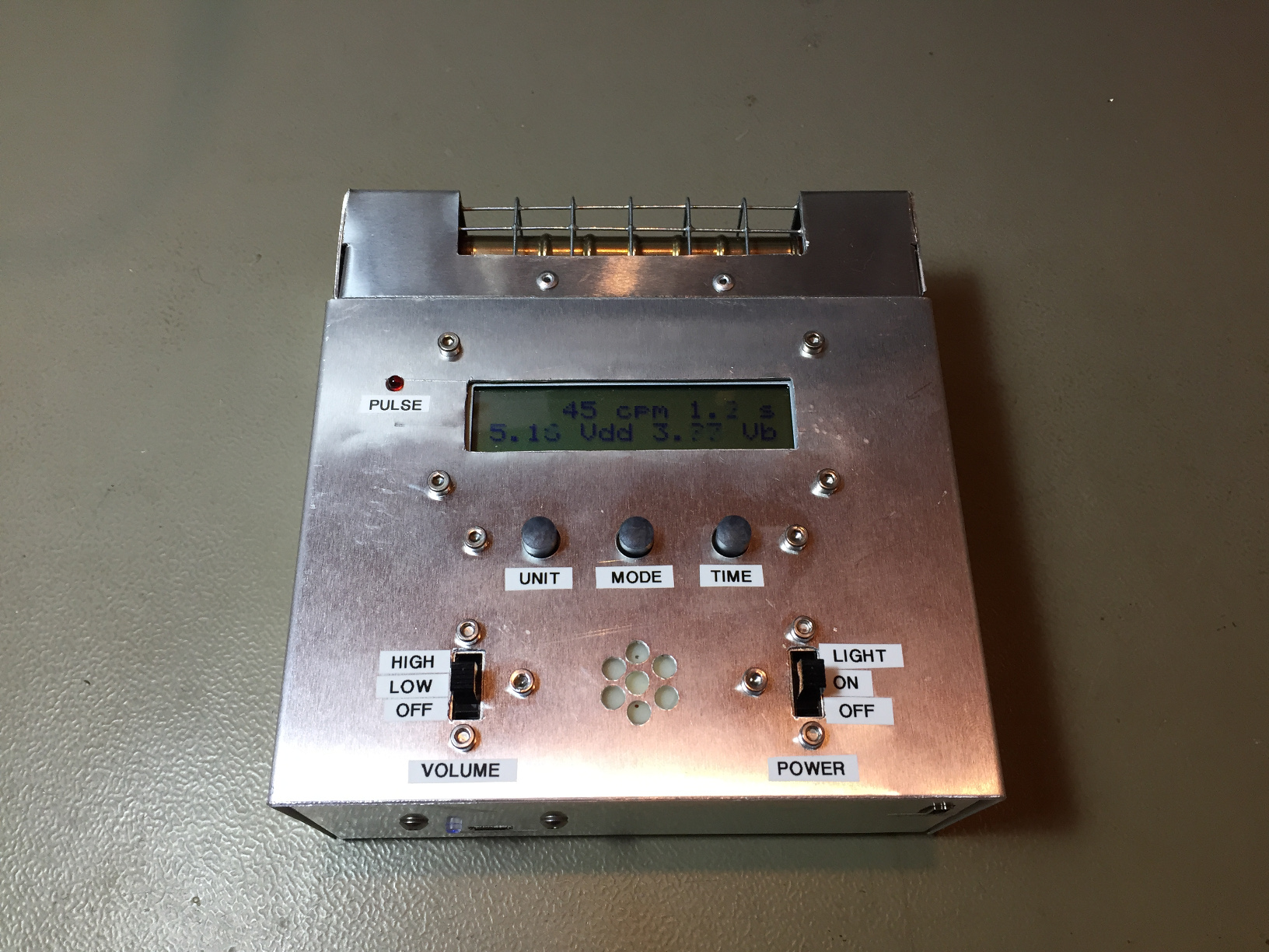
Top view of the finished instrument (click to enlarge).
First of all, background radiation is low. I'm glad it's like that, but this is basically the only radioactivity you'll ever measure, as I never found anyithing really radioactive. So, I wanted an instrument that is quite sensitive to low radiation levels. When measuring only a few counts per minute, one has to wait a long time to have a meaningful reading and it's quite boring. There are tubes that are more sensitive, but they are expensive. So I decided for a compromise and opted for two SBM-20 tubes instead of just one. This doubles the count and makes reading the background radiation more comfortable and precise.
The choice of the SBM-20 type tubes is mainly based on their low price and good availability online. They are of Russian origin and their original cyrillic reference is СБМ-20.
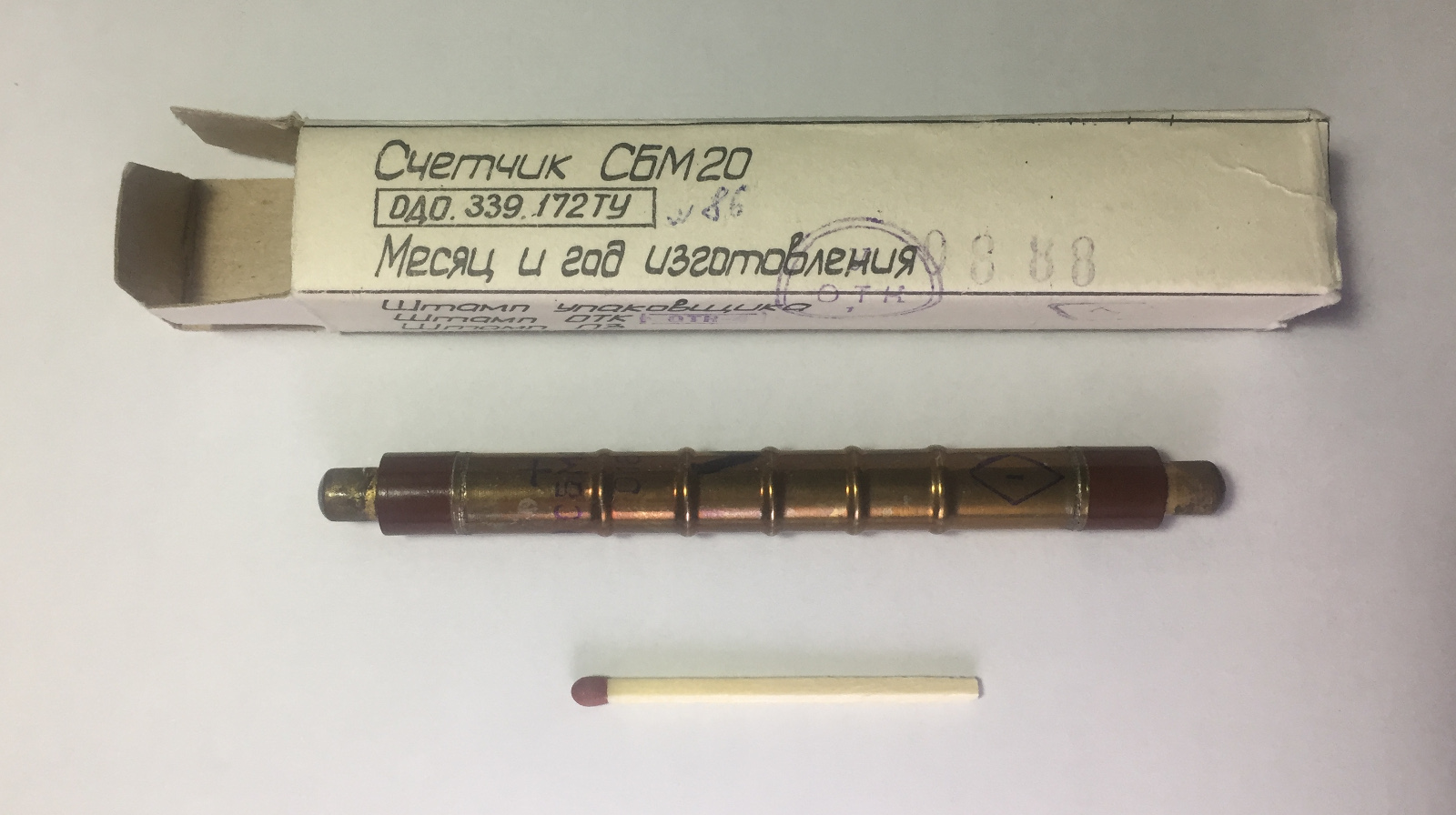
Picture of one SBM-20 Geiger tube and its original package, the match
is for scale comparison (click to enlarge).
My previous counter [3] had a fixed integration time, but I found that uncomfortable. If you want a precise reading you want to select a longer time. If you want a quick reading at the cost of some precision, you want to be able to select a shorter time. I decided to go for 2 seconds, 10 seconds and one minute. Another important point is to display the remaining time during each integration in real-time, otherwise it's difficult to see when a new value is replacing the old one, especially when integrating for a long time. I also wanted some statistical functions like minimum, maximum and average.
Some counters measure in μR/h, some others in nSv/h, and if you're just comparing readings of your own counter, I prefer to count the "ticks" (counts) per minute. So I also wanted to be able to select the unit it can display between these three.
The SBM-20 is rated to work with radiation between 14 μR/h and 144 mR/h. Converted into counts per minute this gives from 21.4 cpm to 220'000 cpm, or frequencies between 0.3 Hz and 3.7 kHz.
Finally, my old counter had the tube installed inside a plastic container and this shielded the radiation quite a bit. Even if I thought that radiation goes through many materials as if they were transparent, I remarked that the values I measured were lower with the box closed. Since I wanted a sensitive instrument for low radiation values, I had to take care of how to mount the tubes, avoiding shielding as much as possible.
A Geiger-Müller tube (very often called just "Geiger tube", sorry Mr. Müller) is a sealed container fitted with two electrodes and filled with a low pressure gas mixture. It usually has the form of a metallic cylindrical tube that is also the cathode (negative electrode). The anode (positive electrode) is in the center along the axis of the tube and is electrically insulated from the tube walls. The gas inside has a fairly low pressure (about 0.1 bar) and is usually a mixture of a noble gas and an organic or halogen vapor. The tube has at least one very thin wall to allow ionized radiation to enter with minimal attenuation: either the tube wall itself is thin or it has a thin end cap, often made with mica. Because of the thin wall and of the low internal pressure, the tube is very fragile and easily breaks if pressed too hard: it must be handled with care.
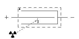
Simplified structure of a Geiger-Müller tube.
A high voltage is applied on the tube electrodes to generate an internal electric field in the gas. Normally, the tube is not conducting and no current goes through it. When an ionized radiation enters the tube, avalanche in the gas takes place and for a short time the gas ionizes and conducts, allowing a pulse of current to go through. Then, the ionization ceases and the tube becomes non-conducting again.
The avalanche in the gas greatly amplifies the little charge caused by the ionizing radiation and is often called "gas amplification". It allows good sensitivity but completely loses information on the particle that generated the pulse. In a Geiger counter, all pulses are alike, regardless of the kind of particle that was detected and its energy.
By counting how many pluses occur in a given time, the ionization can be determined. Usually the frequency of the pulses is given in counts per minute (cpm). The pulses arrive randomly to the tube, so a suitable integration time has to be selected in order to determine their frequency. If the integration time is too short many readings will be zero, if it's too long it will be boring to wait for a valid reading. In order to have more precise readings at low radiation levels, this Geiger counter uses two tubes.
The operating voltage is very important and it's always specified in the tube datasheet. If it's too high, once ionized, the tube will stay ionized and will never deionize to detect any further radiation. If it's too low, the tube loses sensitivity and measure less than what it should, if it measures something at all. Fortunately, the operating range is quite wide and not too critical as far as the limits are not exceeded. For example, the SBM-20 works from 350 to 475 V, with a recommended operating voltage of 400 V.
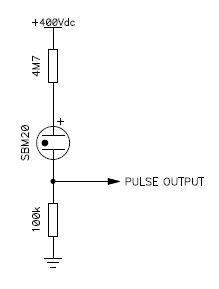
Basic Geiger tube connection.
A series resistor to limit the current is mandatory. A low resistor value shortens the dead time but if it's too low, the current in the tube will be too high and the tube life will be affected. If it's too high, the tube will take more time to react and loose some sensitivity when dealing with high radioactivity levels. The SBM-20 datasheet recommends a 5.1 MΩ series resistor for normal operation and an absolute minimum resistor of 1 MΩ. Since I didn't have any 5.1 MΩ resistors, I used 4.7 MΩ instead. To count or integrate the current pulse provided by the tube, the easiest method is to put a series resistor in the tube ground connection, so that a low voltage pulse appears across it. Then, it can be easily processed by common logic ICs. More information on Geiger tubes can be found in [6].
When a radioactive particle strikes the tube, the gas is ionized and a pulse is generated. Then the ionization disappears and the tube is ready again for the next particle, but as long as it's ionized, it cannot detect another particle. This is called dead time and de facto shortens the integration time. Every time the tube generates a pulse, for the whole duration of the pulse, the tube is "blind" and cannot see another particle should it come during that time. You can see dead time as a "processing time" the tube needs to "handle" the particle; while busy, it cannot detect another particle. The more pulses are counted, the more time the tube is blind (dead). This is easy to compensate with just a simple formula that considers a shortened integration time due to all the detected pulses. If f is the measured pulse frequency and τ is the tube dead time, the corrected pulse frequency f' can be expressed as follows:
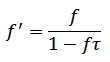
Of course, time units for f and τ must match. Since usually f is expressed in cpm (counts per minute) and τ in microseconds, a unit conversion has to take place. More information on tube dead time can be found in [6].
The SMB-20 tubes used in this project have a dead time of 190 μs and a maximum frequency of 220'000 cpm. The correction increases as the count increases, and the correction makes the reading even higher. For example, for this tube, the correction is about +1 % at 3'000 cpm, +10 % at 30'000 cpm and +50 % at 160'000 cpm. At low radiation levels of just a few tens of cpm, the correction is small and can be neglected.
This counter is intended to measure low values of radiation, so dead time will probably never play a significant role in the accuracy of the measurements, but since this equation is very easy to implement in a microcontroller, it would be a pity not to do it.
In order to power the Geiger tube, a high voltage is required. For the SBM-20 tubes we need 400 V. Others tubes usually require between 350 and 500 V. Designing a step-up converter that is simple, reliable, cheap and stable is by far the most difficult task. I tried several designs and I got it right at the third attempt. First I tried with a simple C-MOS IC oscillator driving a power MOSFET and a simple inductor. This didn't work very well; the voltage on the inductor was too low, probably because the edges of the signal weren't sharp enough. I than tried an LT-1070 which is a true step-up DC-DC IC also driving a simple inductor. This worked somehow better, but still the voltage wasn't high enough. I could have solved the problem by replacing the inductor with a transformer or by adding a voltage multiplier at the output, but I was not convinced it was the way to go. The circuit was already complicated enough, the IC is quite expensive and I was too lazy to design and build my own transformer.
While thinking on where to find a suitable transformer, I stumbled upon an old disposable camera flash unit. It has a nice little circuit capable of converting the 1.5 V of a single AA cell into the 300 V required by the flash tube. In its simplest form, it has a transformer, a transistor, a diode, a resistor and a capacitor. It could not be simpler. It's very cheap because is supposed to be disposable. And it's very reliable as well because it's manufactured in large volumes.
Unfortunately, I didn't take a picture of that particular unit before taking it apart, but just to give an idea, here is a picture of a similar unit, with a different looking transformer, but the circuit is almost the same.
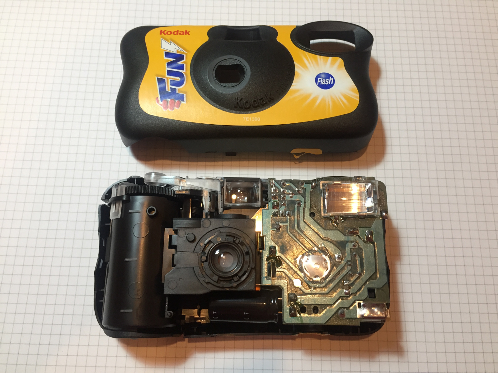
Two pictures of a disposable camera, where a suitable transformer can be
found.
Unfortunately, this is not the same one I used to salvage my transformer and
it looks a little different (click to enlarge).
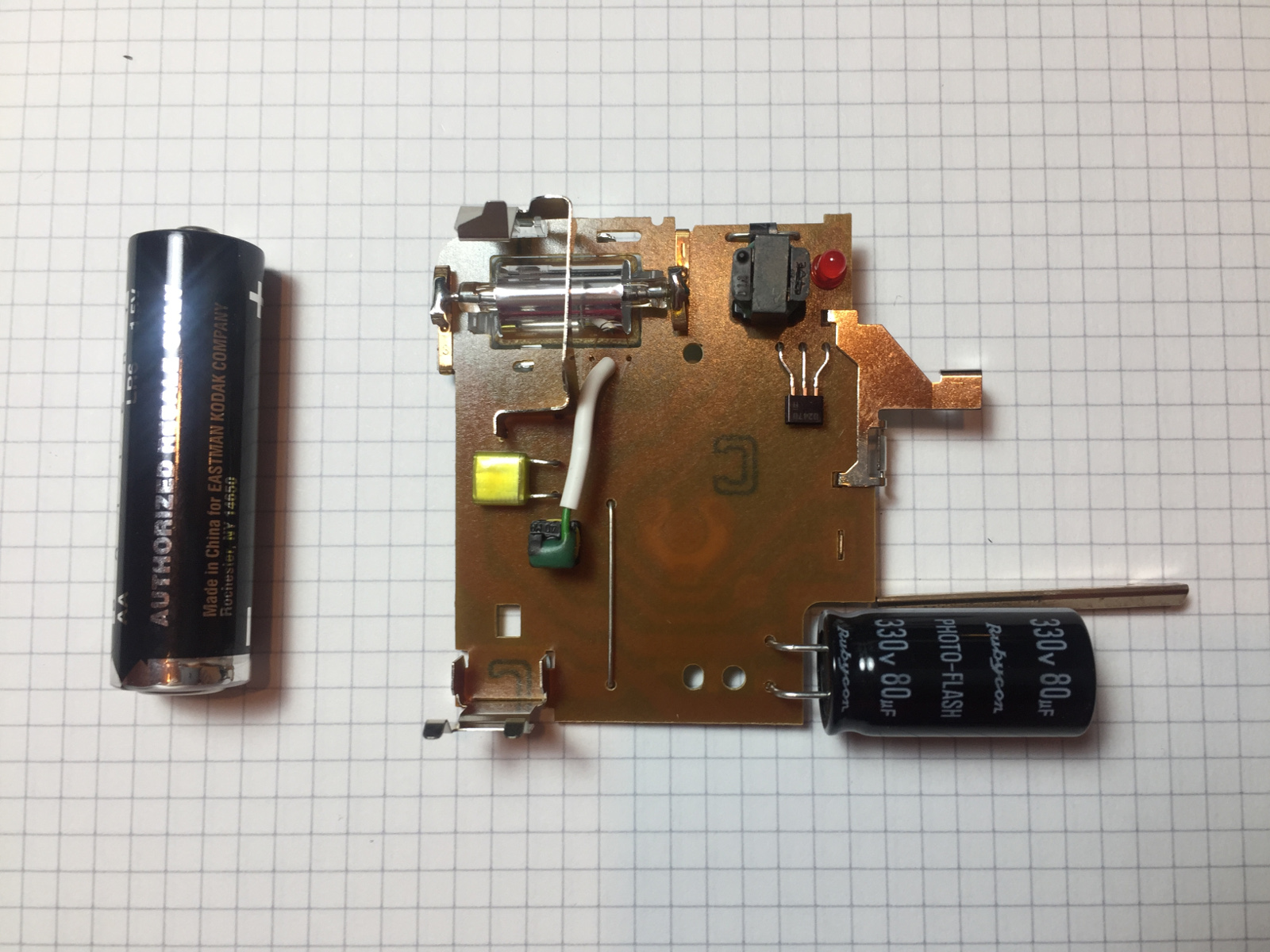
I started by reverse-engineering the unit I had. The circuit diagram is represented below and is quite a deluxe version as it also has and LED to indicate when the capacitor is charged:
Original circuit diagram of the disposable camera where the
transformer was found.
As it is, it will not do the job. I wanted to power the whole instrument with 5 V which is a convenient value; 1.5 V is too low for a microcontroller and an LCD display. And I also needed a higher output voltage, but I was sure the transformer will work: it has a suitable turn ratio, it's well insulated and can be easily sourced for very cheap.
While being extremely simple, the circuit is very interesting. It's a one transistor, self-oscillating blocking oscillator. This is not a resonant oscillator; the oscillation is due to the saturation of the transformer. Since the transformer is designed to saturate, it's suitable for such a circuit and will perform well.
Before going forward, I would like to warn you about the dangers involved with high voltage. Even a simple disposable camera can be dangerous. The charge in the electrolytic capacitor can last for a long time after the battery has been disconnected. Always discharge the capacitor before touching with your hands and make sure it cannot charge again. It can hurt really badly and maybe even be lethal. Continue only if you know what you're doing and at your own risk.
This being said, I started by simplifying and modifying this circuit for my purpose. I removed the pushbutton used to charge the output capacitor as this unit will work continuously. I also removed the LED which makes no sense anymore. I added a 47 μF filter capacitor on the power supply to provide a local energy storage and avoid large current pulses on the supply line. I increased the value of the resistor to cope with the higher supply voltage and I drastically reduced the value of the output capacitor from 80 μF to just 10 nF. This is very important as Geiger tubes are high impedance devices and do not require a big energy storage capacitor. By reducing this capacitance, the risk of electric shock is greatly reduced: it will still bite your finger if you touch it, but won't hurt as bad. I was extremely careful with the original 80 μF capacitor, but I touched by accident the 10 nF one: it "woke me up" real quick and made me more careful for the next time, but nothing really bad happened.
Often these simple flash units generate a negative high voltage, but I needed a positive one. Simply reversing the diode is not a good idea, because we don't have a symmetrical waveform. So I connected two diodes in different directions to experiment which one gave the best result.
The test circuit is visible here:
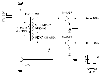
Test circuit of the high voltage generator to determine winding phase
and configuration.
You may remark that I used a different transistor. This is because I inadvertently blew up the original one. This circuit will eat your transistor if you're not careful enough. Running it with no diode connected on the secondary or letting it draw too much current are very bad ideas. So I ended up with a more rugged transistor I found in my junk box.
Let's have a look at how it works: suppose that you just switched on the power. The transistor is off (blocked) and there is no collector current. A small current flows through the reaction winding and the resistor turning the transistor on. As the transistor turns on, the induced current in the reaction winding will turn it on even more. The collector current will rise until the transformer will saturate. This reverses the induced current in the reaction winding switching the transistor off. The magnetic flux in the transformer will collapse and a high voltage surge appears at the secondary. Actually, the pulse appears on all windings, but on the secondary it has the highest voltage because of the high turn ratio of this winding. Once the flux has gone, the whole cycle repeats. If the oscillator doesn't work, reverse either the primary or the reaction winding (but not both). It's called a blocking oscillator because the transistor is oscillating between being completely blocked and fully saturated, instead of being in its linear region as in a resonance oscillator.
The voltage on the secondary depends on how quickly the transistor turns on and off and can hardly be calculated (as far as I know). By measuring the voltage rectified by the two diodes, I found +400 V and −600 V. A higher negative voltage makes sense, as this circuit was originally designed to produce a negative high voltage, so simply reversing the diode will not work well. This is because this circuit is a fly-back converter: it utilizes the collapsing magnetic field when the transistor turns off to generate the high voltage output. The pulse of opposite polarity when the transistor turns on is not desired and is only a stray effect.
Reversing the secondary would work, but it's internally connected with the reaction winding and cannot be separated, so the trick to have a positive output voltage is to reverse both the primary and the secondary/reaction windings: the phasing between the primary and the reaction windings will not change (the oscillator will still work as before), but now the secondary winding is reversed, as well as the polarity of the output voltage.
When measuring this voltage, it's important to use a high impedance voltmeter, such a digital multimeter with an input impedance of 10 MΩ or more. A low impedance instrument would load this generator and read too low. It could even stop the oscillator completely if the impedance is really low.
This is the final configuration:
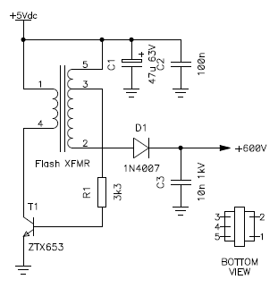
High voltage generator design before adding voltage regulation.
The choice of the resistor is important. I tried several values until determining that 3.3 kΩ was the best compromise. You want a resistor that is high enough to avoid stressing the transistor too much, to keep it cool and keep the power consumption down. But you have to make sure that the resistor is low enough so that the oscillator can start reliably, even when the supply voltage is lower than usual and when the output is fully loaded. In my tests I considered a minimum supply voltage of 4 V and I loaded the output with a 2.2 MΩ resistor to ground. This simulates a discharged battery and a condition where the two tubes conduct at the same time (each one is connected with a 4.7 MΩ series resistor). This is probably a worst case scenario, but gives some margin for a reliable operation.
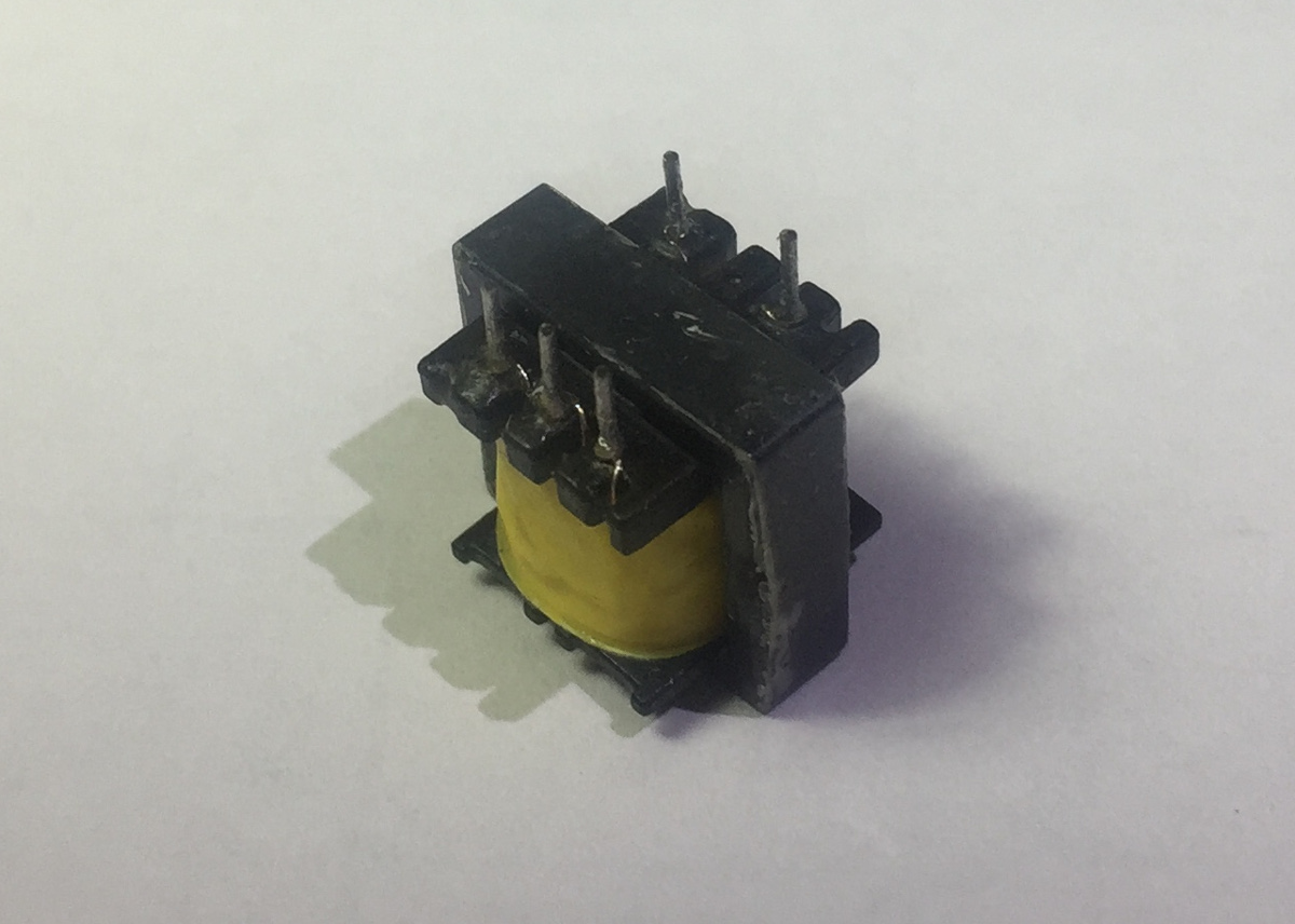
Picture of the transformer used in this circuit (click to enlarge).
The main component of this circuit is the transformer, which is also the more critical. It's something which is not easy to by new, but you can salvage it from a disposable camera, probably for free. Other potential sources of suitable transformers are bug zappers, small cobra flashes and CCFL (cold cathode fluorescent lamps) power supplies as the ones used for LCD backlight in some laptop computer. Once you have the transformer, you can start reverse engineer the original circuit to see if and how it can be converted into a proper Geiger counter high voltage power supply.
The windings configuration of common camera flashes is quite strange: the reaction and secondary windings are internally connected in series. If I designed the transformer I would probably considered three independent windings, or the primary and the reaction together and a separate high voltage secondary. But at the end, this is not really important as the circuit works fine. I don't know why camera manufacturers choose this configuration. Because the secondary side has a much higher voltage and a much lower current than the other two windings, it doesn't really matter if it's connected to the +5 V rail or to ground, neither if its current flows through another winding as well.
The table below summarizes some of the measured parameters of the transformer used here. It's just reported as a curiosity, as a different flash transformer will probably work just as well. One just has to spend some time in identifying the different windings and their phase by swapping the terminals until the oscillator works and produces the desired output.
| Winding | Terminals | DC resistance | Inductance | Turn ratio |
| Primary | 1-4 | 0.2 Ω | 1.41 mH | 1 |
| Secondary | 2-3 | 170 Ω | 4'610 mH | −1:57.2 |
| Reaction | 3-5 | 0.2 Ω | 0.29 mH | 2.14:1 |
There is one more thing to do to complete this block: add a feedback circuit to stabilize the output voltage. This is done by transistor T2, as represented in the figure below, which is the final circuit. I selected a Darlington transistor for this task, because I wanted to minimize the load on the transformer output. Darlington transistors have very high gain and therefore require only a very small base current.
The output voltage is first reduced by two Zener diodes in series, dropped into two 10 MΩ resistors and a trimmer, and fed into the base of T2. When the voltage here rises above its conduction threshold (about 1.2 V) T2 starts conducting and robs current from the base of T1. This results in reducing the current in the transformer and therefore the output voltage.
There is nothing magic about the two Zener diodes in series, it's just because I didn't have a single 300 or 350 V Zener in my junk-box, so I had to connect two in series. The two 10 MΩ resistors in series are because 10 MΩ is the highest common value available and I needed about 20 MΩ to keep the load current down.
The 100 pF capacitor across one of the two 10 MΩ resistor was determined experimentally to improve the response of feedback circuit to variations on the load. With this capacitor the response is a bit faster, but it's not a critical part and since a Geiger tube draws very little current, the circuit will work fine even without it.
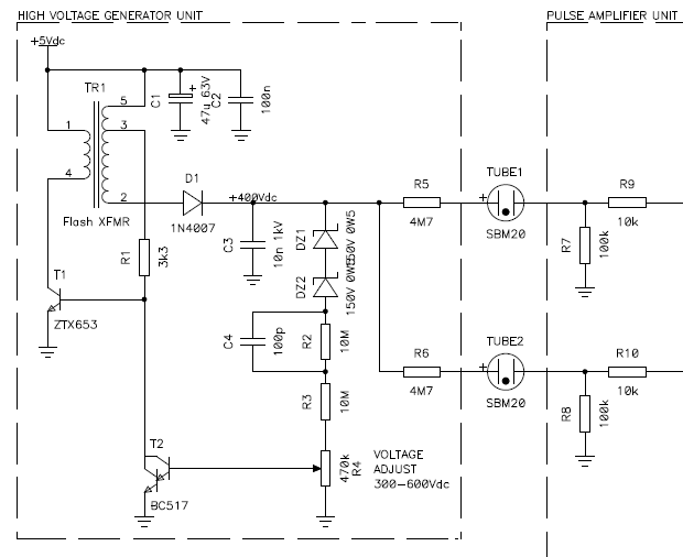
Circuit diagram of the high voltage generator unit, also showing the
two Geiger tubes and the input section of the pulse amplifier unit (described
later).
The assembled module is visible below. Since I had to experiment quite a bit on this generator, I decided to use a "dead bug" style of construction instead of drawing, etching and assembling a PCB. I'm glad I did it that way; otherwise I would have built it three times... Especially playing with the phase of the different transformer windings made me swap several times the connections. At the end, I decided to keep it like that. Of course, it could be built on a nice PCB, but I didn't see the need of building it again.
When done testing and assembling the circuit, I finally adjusted R4 to have 400 V on the cathode of D1, again using a high input impedance digital multimeter.
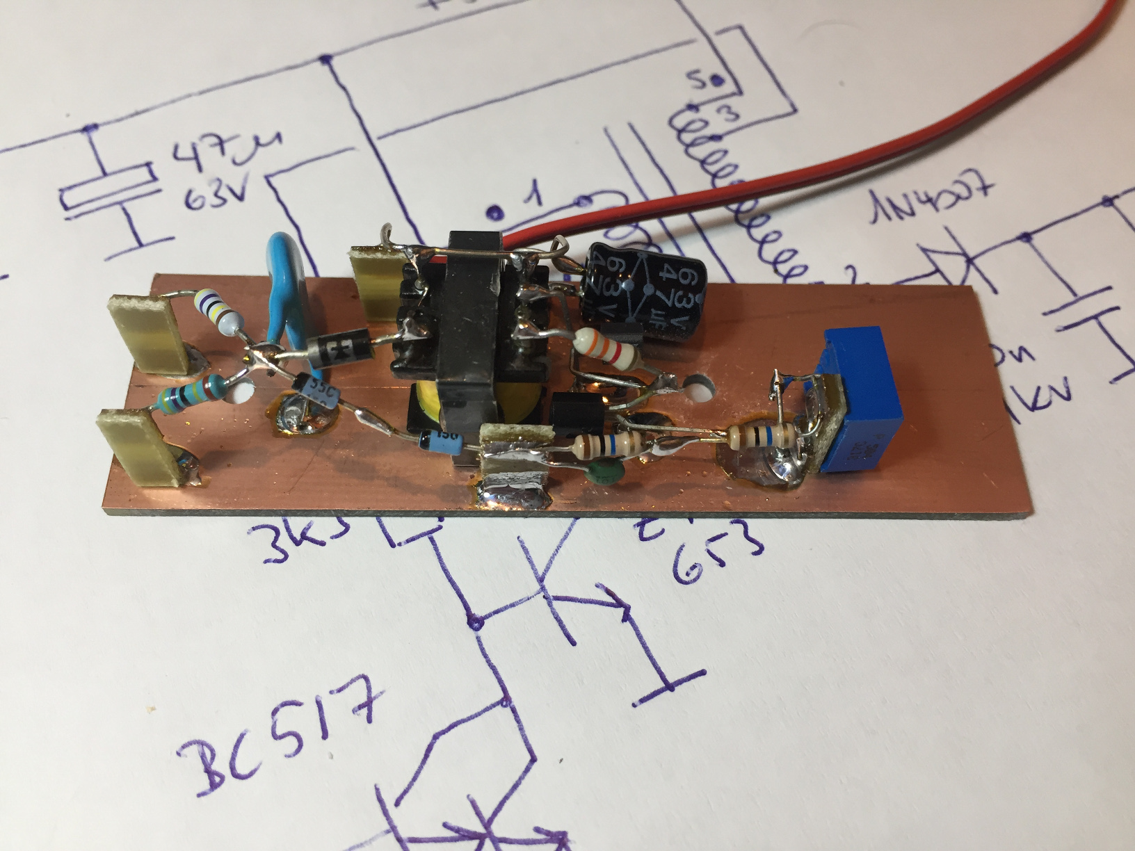
Picture of the high voltage generator module (click to enlarge).
I also connected an oscilloscope to see how the oscillator was performing. The frequency of operation is around 10 kHz and decreases a little bit when loaded. When regulated for +400 VDC, the output winding (transformer pin 2) swings between −300 V and +400 V. The peak positive voltage is produced while T1 is turned off, confirming that this circuit works as a fly-back converter.
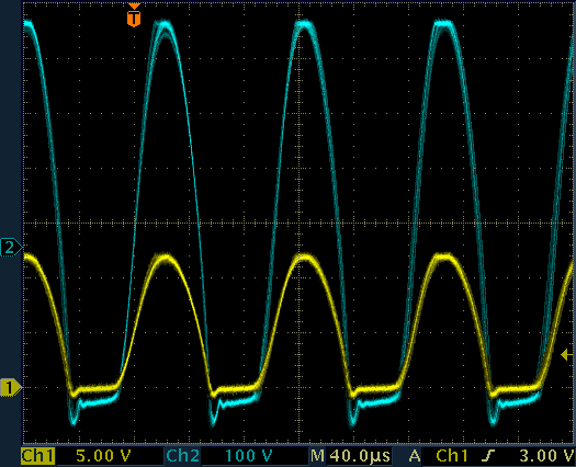
Waveforms on the high voltage generator.
CH1: transformer pin 4, CH2: transformer pin 2.
No load on the output.
Please observe in the figure below that the voltage on the feedback winding (CH2) is (of course) 180° out of phase in order for the oscillator to work. Please also remark how the voltage on the primary (CH1) swings well beyond the power supply voltage of 5 V, reaching 12.5 V while the T1 is turned off.
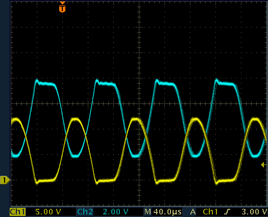
Waveforms on the high voltage generator.
CH1: transformer pin 4, CH2: transformer pin 3.
No load on the output.
When heavily loaded, the oscillator struggles to keep the regulation and its frequency becomes a bit unstable, but it's still working fine. Here it's loaded with 2.2 MΩ to ground, which is a worst case scenario.
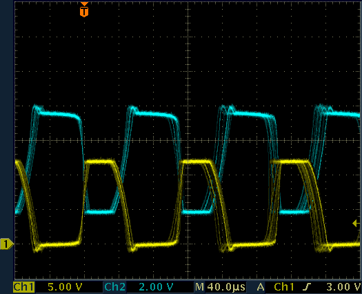
Waveforms on the high voltage generator.
CH1: transformer pin 4, CH2: transformer pin 2.
Output loaded with a 2.2 MΩ resistor to ground.
I named this section "pulse amplifier" but I should rather have called it "pulse shaper" or "pulse level shifter". The goal is to convert the tiny analog pulses provided by the tubes into logic level pulses a microcontroller can count.
Many commercial multi-tube Geiger counters simply connect the tubes in parallel. This works, but I wanted to be able to count the pulse of each tube separately, so I equipped each tube with its own pulse converter. I wanted to be able to handle the situation when both tubes detect a particle at about the same time: if the tubes are in parallel, you only see one pulse; if they are separated, you get a pulse from each. One may argue that in this case the same particle probably crossed both tubes at the same time. Should it be counted only once? I don't know, but this can later be sorted out in the microcontroller. For this counter, I decided to count all pulses, regardless if they are simultaneous or not. Counting the pulses separately has also the advantage of showing if one tube suddenly has a problem and stops working.
Anyway, the current pulses provided by the tubes are converted into voltage pulses by resistors R7 and R8. Their value is selected so that the maximum voltage (when the tube behaves like a short circuit) only slightly exceeds the 5 V power supply. With a +400 V tube supply and a tube series resistor (R5 or R6) of 4.7 MΩ, using 100 kΩ for R7 and R8 gives a pulse of maximum 8.3 V. Should you use tubes with a significantly different high voltage supply or series resistor, you may need to adjust the value of R7 and R8 accordingly.
These pulses are fed into two Schmitt-trigger inverters that will square the pulses and provide a nice low impedance output. Resistors R9 and R10 protect the inverter inputs from voltages above or below the supply rails. All logic inverters of the C-MOS 4000-series IC have internal protection diodes that clamp the input to the supply rails, but a series resistor is necessary to limit the current and protect the diodes themselves. No external additional diodes are required. Here I used a CD40106B hex Schmitt trigger inverters simply because I had plenty in my junk-box.
It's important to keep the stray input capacitance of this amplifier as low as possible. Pulses are weak and will disappear if they have to charge a large capacitance. So, mount the amplifier very close to the tube. If you want to mount the tube remotely from the rest of the meter, say at the end of a cable even only one meter long, you should put the amplifier next to the tube and send the amplified signal through the cable.

Circuit diagram of the pulse amplifier unit, also showing the two
Geiger tubes and the output section of the high voltage generator unit
(described before).
The outputs of these inverters are 5 V TTL compatible and are fed directly into the microcontrollers (connections labelled "TUBE1" and "TUBE2"). Pulses are of course inverted, so the voltage is normally 5 V and drops to 0 every time a particle is detected.
Pulses are also combined together by D2, D3 and R11 that form a discrete AND gate. This is used to generate a "tick" sound, typical of a Geiger counter and also to flash an LED at the same time. For this acoustic and visual effect, the pulses of both tubes can be simply combined together, as the goal is only to give a rough feedback and not a precise measure. I have to say that the ticking sound is a very handy feature because it gives a feeling of the reading without even looking at the display, you just hear if there is a sudden increase or decrease of the measured value before the integration time is actually over.
For the ticking sound, the pulses go through two consecutive inverters U1:E and U1:D, drive transistor T3 and a small speaker. These two inverters are not strictly needed, but they are part of the IC anyway, so there is little reason not use them to drive the base of T3. The speaker was salvaged from and old cordless phone. It's small, rugged, not too loud and has a high impedance (140 Ω). I included a switch (SW1) to decrease the volume and to mute the sound, if necessary. The reduced volume is obtained by putting R14 in series with the speaker. Its value was experimentally determined until I got the volume I wanted. This circuit will work with any speaker, even common 4 Ω or 8 Ω speakers, but you may need to play with the value of R14. I like the high impedance of this speaker because it draws little current from the supply rail, but this is not really important as capacitor C7 provides a local energy storage to keep the supply voltage clean. Diode D5 works as a flywheel and absorbs high voltage spikes generated by the inductance of the speaker.
I tried to feed the pulses directly into an LED, but they are only about 110 μs long and they are too short to be visible. So I used inverters U1:B and U1:C to form a mono-stable circuit and enlarge the pulses to about 2.5 ms. This provides nice bright flashes. If the pulse frequency is too high, above about 400 Hz, the LED will simply stay on.
Oddly enough, I tried to use the enlarged pulses also to drive the speaker, but I didn't get any significant volume change, so I kept the speaker on the original pulse width. This allows the speaker to continue working even with pulse frequencies much higher than 400 Hz.
As it can be seen in the picture below, I also built this section without an etched PCB. Since I only needed one instrument, I didn't bother drawing, etching and drilling; once I was happy with my "dead bug style" prototype, I drilled two mounting holes in the base board and I kept it as is.
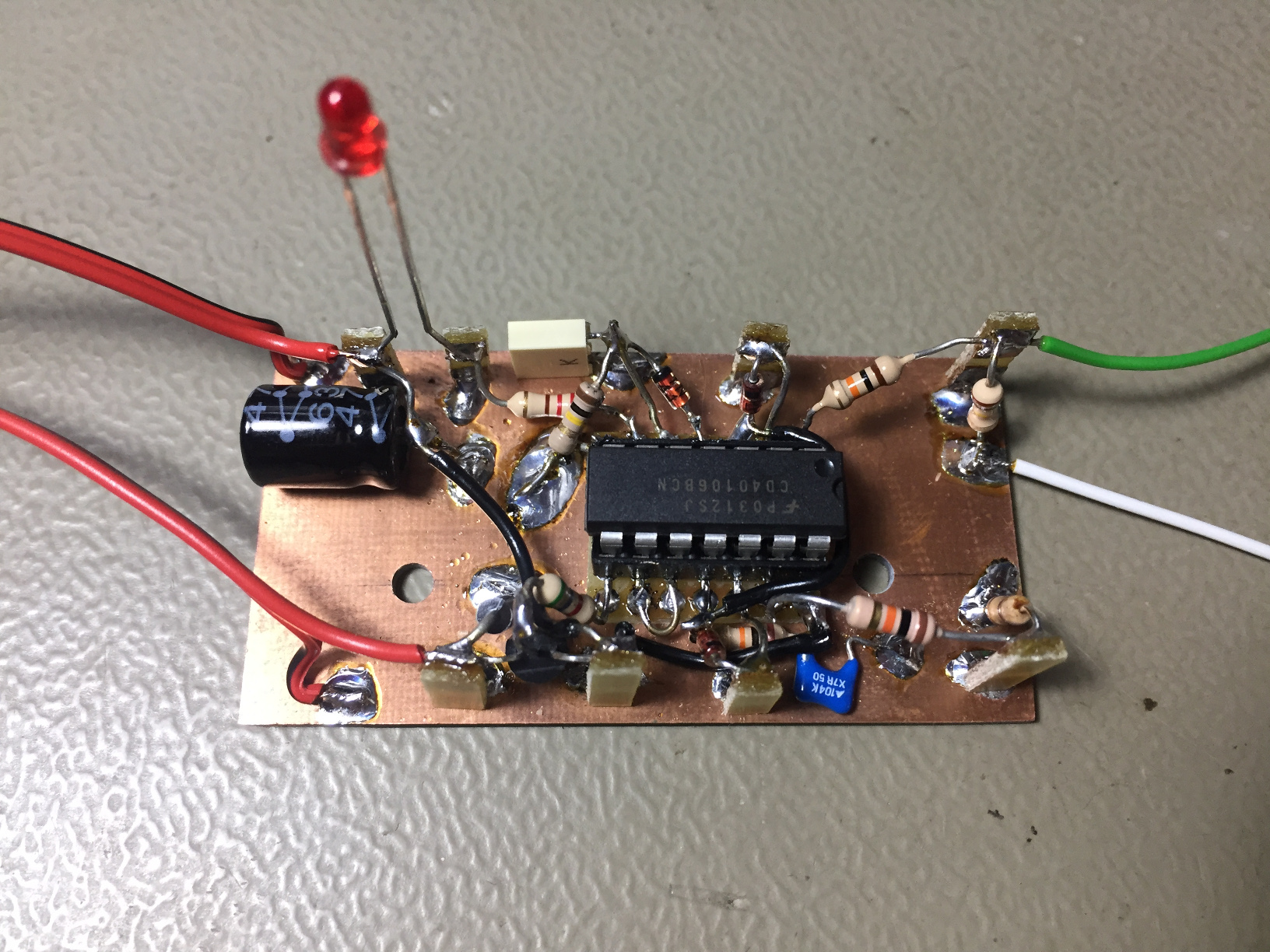
Picture of the pulse amplifier module (click to enlarge).
The following figure shows the pulse generated by the Geiger tube (CH1) measured across the 100 kΩ resistor and the shaped pulse sent to the microcontroller (CH2). The pulse from the tube is a very thin and sharp pulse followed by a larger and lower trail. The total length of this pulse is roughly the dead time.
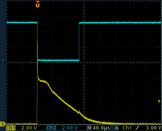
Waveforms on the pulse amplifier.
CH1: Geiger tube cathode, CH2: Arduino pin D2.
In the following figure one can see the enlarged pulse used to drive the LED.
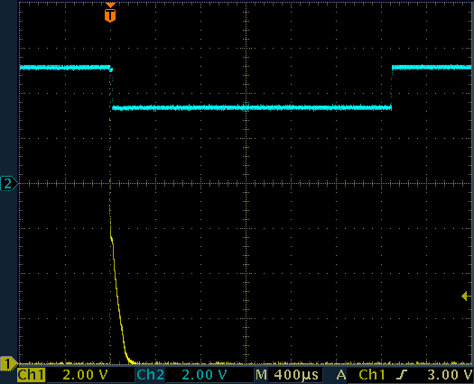
Waveforms on the pulse amplifier.
CH1: Geiger tube cathode, CH2: LED cathode.
Now, by simply connecting this pulse amplifier, the tubes, and the high voltage generator, we already have a working Geiger counter. Just power it with a 5 V supply and it will start ticking. In the next sections, however, we'll have a look at how to display meaningful measurements and how to power the whole instrument with a battery.
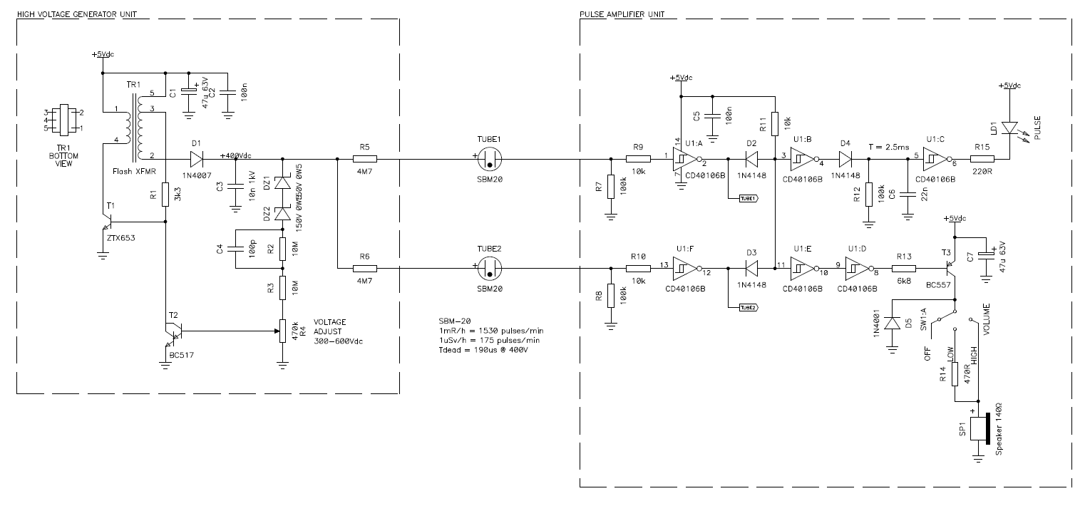
Circuit diagram of the whole analog section (high voltage generator
unit, Geiger tubes and pulse amplifier). If powered with 5 V, this
circuit is enough to detect radiation and make the speaker tick
(click to enlarge).
I called this block "control unit" because it's based on a microcontroller, but strictly speaking, this is more a "display unit" as the previous sections already work fine as a Geiger counter and there is nothing to control.
The heart of this block is an Arduino Nano board, which is basically a PCB fitted with an ATmega328 microcontroller and an USB interface. The pulses from the two tubes are fed into D2/INT0 and D3/INT1 lines. These two lines have independent interrupt capability and this makes implementing two counters in the software a lot easier. By using the hardware interrupt features of these lines, both counts are updated regardless of the load of the CPU and regardless if two pulses arrive at the same time. Because of the inverting characteristic of the pulse amplifier units, these two lines are high when idle.
A 16-character 2-lines dot-matrix LCD display is connected to lines D4, D5, D6, D7, D8 and D9. Trimmer R20 adjust the display contrast and SW2:B allows switching the backlight on or off. Three buttons and one jumper are used to control the instrument. They are connected to D16/A2, D17/A3, D18/A4 and D19/A5 and use the internal pull-up resistors of the microcontroller.
R16/R17 and R18/R19 form two 5.7:1 voltage dividers and are used to read the battery and VDD rail (+5 VDC) voltages respectively. They are connected to D15/A1 and D14/A0. To ensure a reliable reading, the internal 1.1 V reference of the microcontroller is used. This is mainly used to display a low voltage warning when the LiPo battery drops below 2.9 V (see the power supply section below).

Circuit diagram of the power supply unit and the control unit (click
to enlarge).
The program implements the counting functions and unit conversion of this twin tube Geiger counter. Every time a pulse (falling edge) is detected, the corresponding counter is incremented by one. This counter is designed to handle two tubes for increased low radiation sensitivity and will automatically correct the results by dividing the collected pulses in half which results in averaging out both inputs. Should only one tube be installed, shorting D19/A5 to ground will remove this averaging function and the software will work perfectly with just one tube. It doesn't matter which input is used, only the division by two is removed. D19/A5 is only checked at the initialization and cannot be changed during runtime (it makes no sense to hot-plug a tube).
Results are integrated, calculated, converted and displayed on the LCD screen. More details on how this is done can be found in the measurements and conversion factors section. Three buttons are used to control the unit. Button P1 ("UNIT") is connected to D16/A2 and allows changing the unit of the result between μR/h, nSv/h and cpm. Button P3 ("TIME"), connected to D18/A4, allows changing the integration time between 2 s, 10 s and 60 s. Longer intervals give more accurate readings but take longer. A countdown on the top right corner of the display indicates the remaining time before the end of the integration. Button P2 ("MODE"), connected to D17/A3, allows changing the mode of the instrument between maximum, minimum, individual tube counts and battery voltage. Pressing and holding P2 will reset the statistics.
Each time an integration period ends, the display is updated and the raw measurements are also echoed on the serial port at 9600 bps. This is useful if you want to log the radiation over a long period of time. No calculation in mR/h nor μSv/h is done on the serial communication, as this can easily be done by the remote PC, based on the raw data. Tube conversion constants and data format is transmitted at boot time. As a reminder, the SBM-20 tube produces 175 cpm at 1 μSv/h and 1530 cpm at 1 mR/h. Dead time is 190 μs at 400 V.
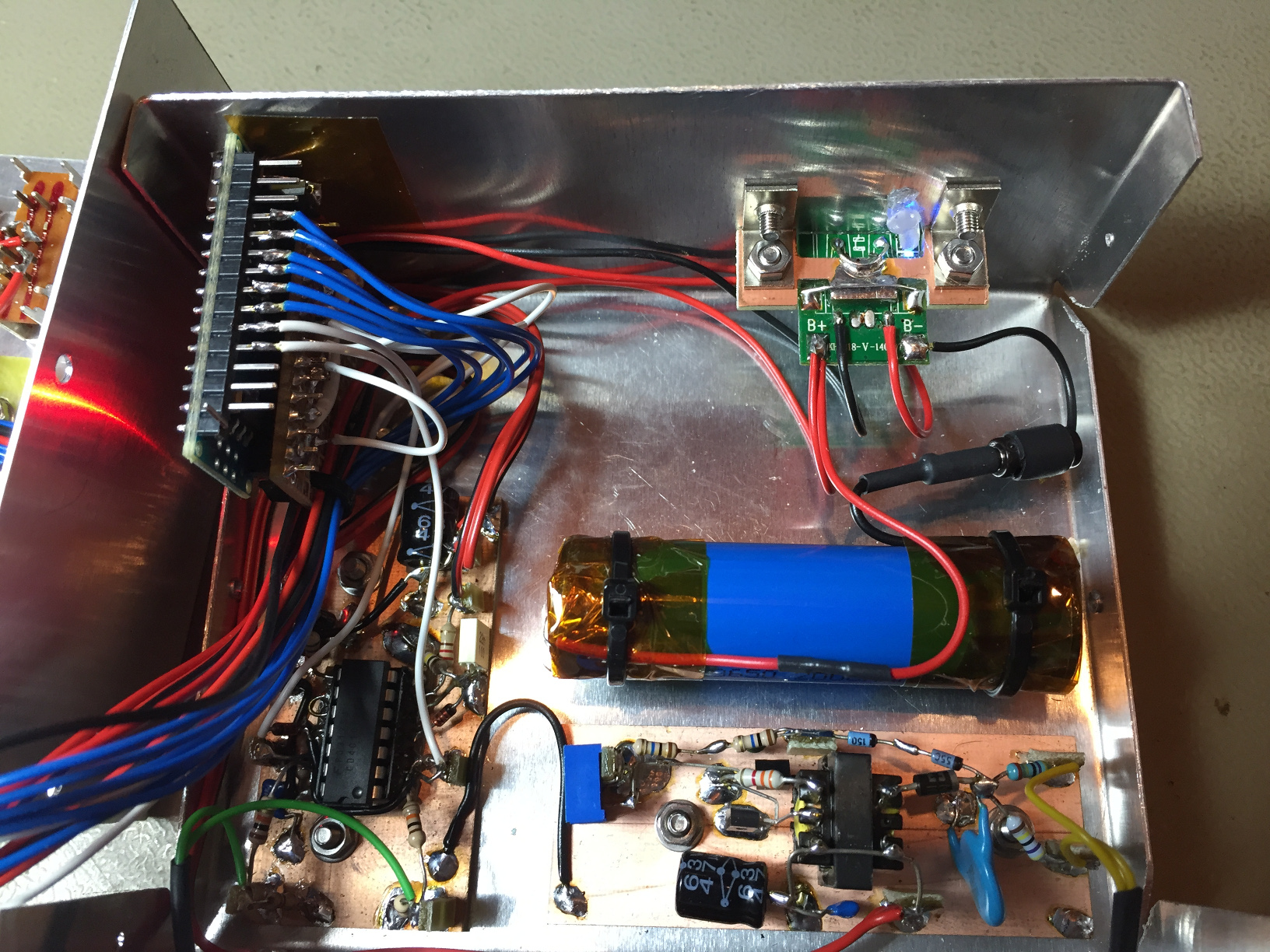
For assembling this part I simply soldered the Arduino board on a pre-drilled proto-board that I use mainly as a mechanical support. The board is bolted to the enclosure with two metal brackets. The few components are "wildly" mounted in the air and there are just a lot of wires going everywhere, so not much to say about them.
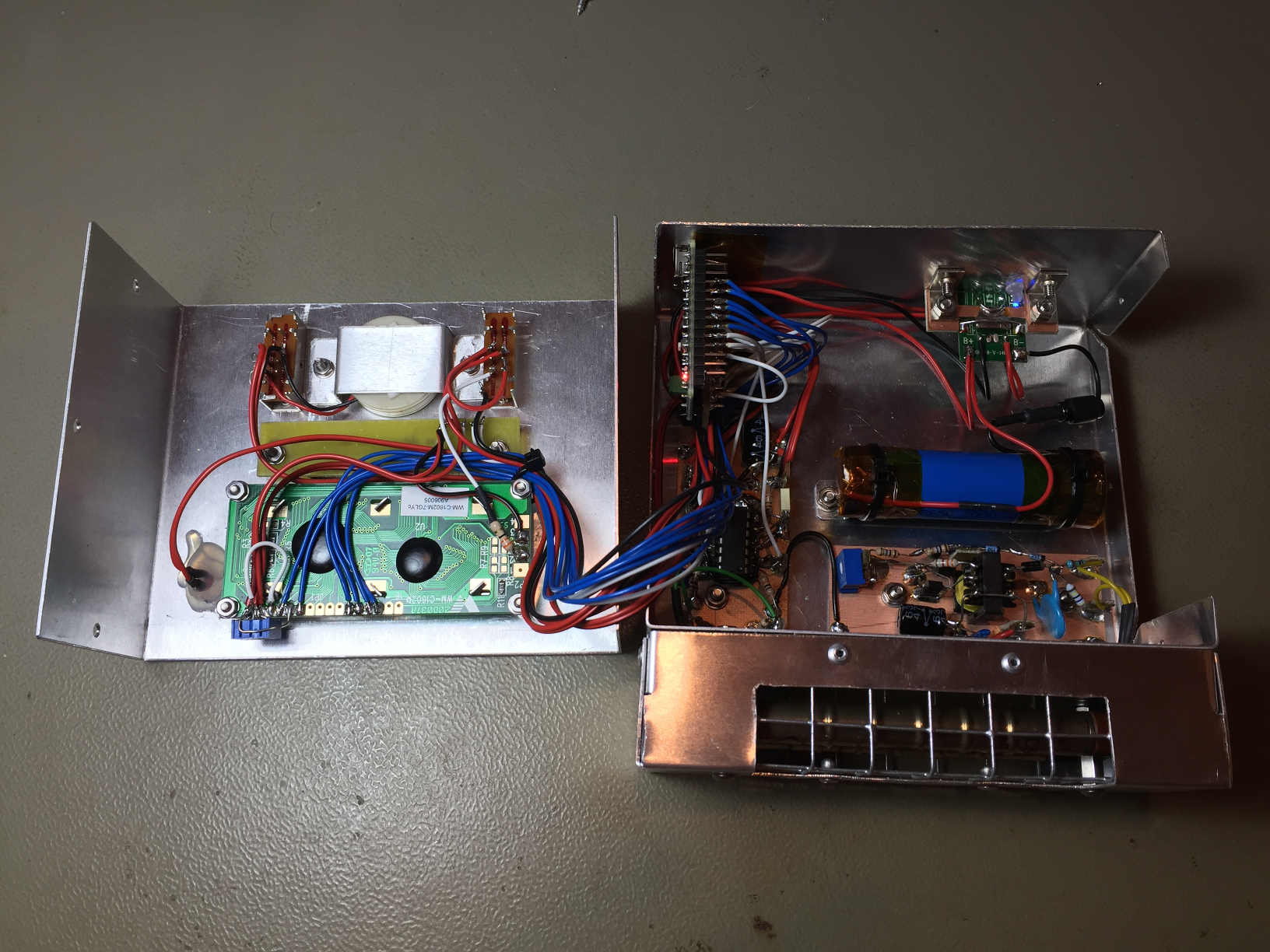
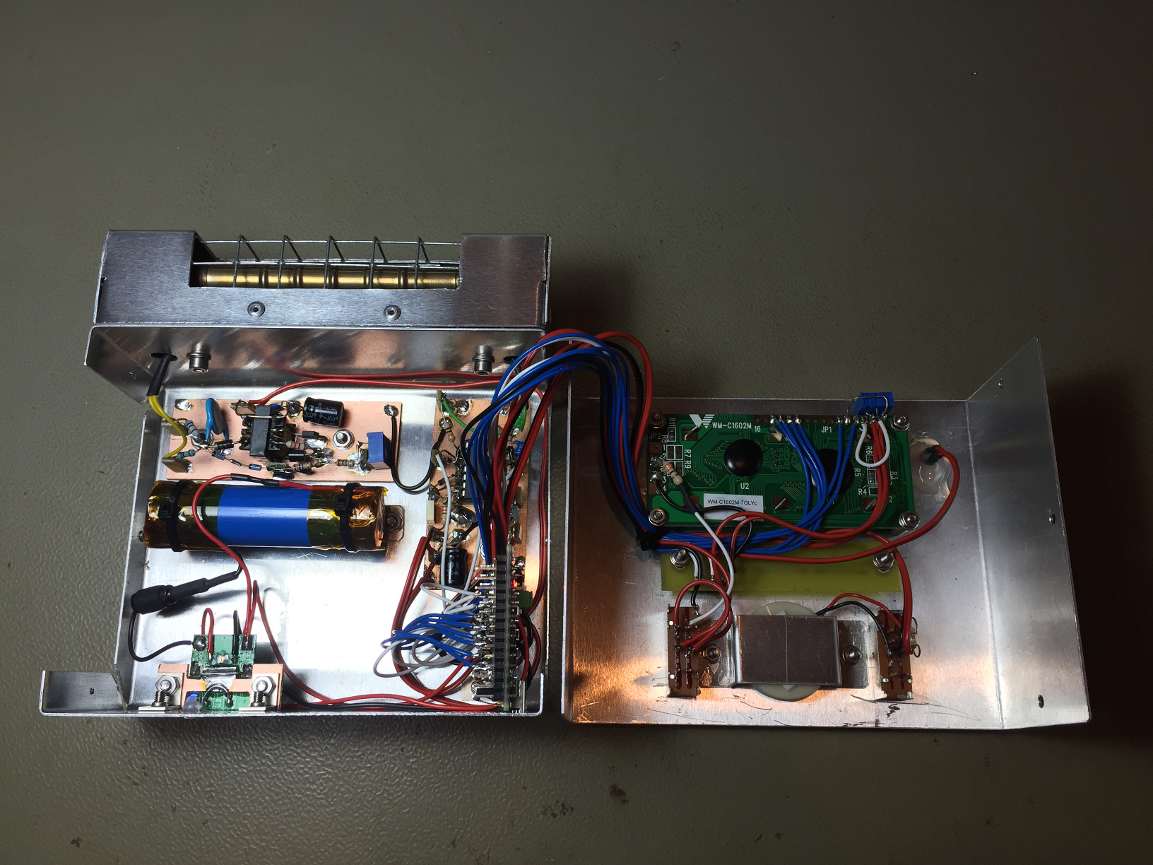
These two pictures show the complete instrument open on the bench from
two different angles (click to enlarge).
If you connect an USB cable to the Arduino, you can power the whole instrument from your PC. This is not the normal way of powering this device, but is useful for developing and debugging.
The firmware (program) used for this application is available here (as freeware): geiger-firmware.zip (9,322 bytes).
Complete PDF schematic diagram: twin-sbm20-geiger-counter.pdf (60,745 bytes).
The first idea was to power with instrument with four 1.5 V AA alkaline cells. Since the nominal voltage of four cells in series is 6 V, a series silicon diode will drop the voltage by 0.6 V and also add polarity reversal protection. This circuit is extremely simple and I used it several times in the past. It has two disadvantages: first, the voltage drop of 0.6 V in the diode is wasted, not allowing using the last 0.6 V of battery voltage when running flat. Second, the voltage slightly exceeds the TTL specifications when the batteries are new, but I never had any issue with it. Knowing this, this circuit is extremely simple and quite a good choice.
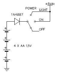
Original idea of a simple power supply with 4 AA batteries and a series diode.
It turned out that I couldn't find a suitable battery holder to go in my metal box. To be more precise, I couldn't find one at a reasonable price. I didn't want to pay more than the price of a Geiger tube for holding four AA cells.
So, why not to power the whole unit with a LiPo battery, like in all modern devices? LiPo batteries are easy to find and are cheap. But the voltage of the cell itself is a bit on the low side and changes with the charge in the battery, requiring a step-up DC-DC converter. LiPo cells also require a dedicated battery charger, because their chemistry is very sensitive and can easily be damaged if charged incorrectly.
While I was thinking about building a battery charger and a DC-DC converter, I stepped into an USB power bank I received for free as advertising. It's actually exactly what I needed: a LiPo charger, an 18650-type LiPo cell with included electrical protection and a DC-DC converter to power USB devices at 5 V.
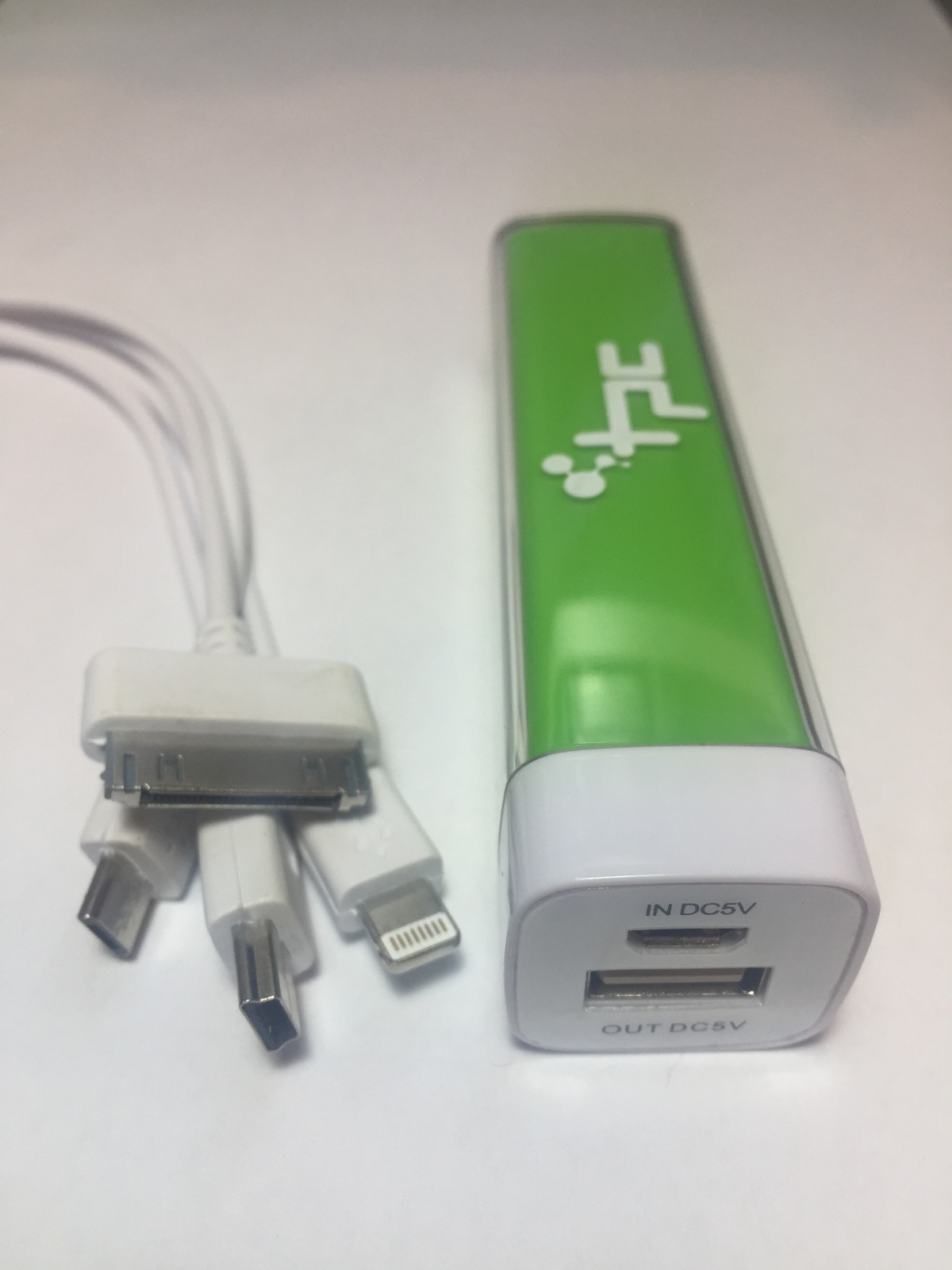
The power bank used to source the battery and the power supply board
(click to enlarge).
So I broke it open and salvaged its guts. It has a tiny PCB with the charger and the DC-DC. It's a bit on the cheap side as the charger uses a linear regulator and the DC-DC is always powered on even when the load is cut off, but it works fine enough.
Having the power-bank PCB already assembled, make the final circuit extremely simple as well, as it can be seen in the picture below:
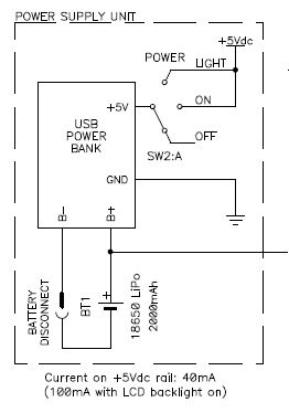
The final LiPo battery power supply circuit using a salvaged power bank.
The connection on the positive lead of the battery going out of the figure is for monitoring the battery voltage from the Arduino and display a warning when the voltage drops below 2.9 V.
Since the battery was soldered directly to the power bank PCB with two wires, it couldn't be easily disconnected, and this can be a problem when working on the instrument as there is the risk of an accidental short circuit and a LiPo cell can provide quite a large current and easily make some damage. So, I installed little connector on the negative lead of the battery and insulated it with heat-shrink tubing to make sure it cannot accidentally make contact with the metallic enclosure. So, when I need to tamper with this part of the circuit, I have an easy way of disconnecting the power. I choose to put the connector on the negative lead so that, if it did accidentally touch the metallic case (which is normally at the same potential), it won't short the battery.
If you wonder why I didn't cut the battery completely out of circuit when the instrument is powered off, it's because in this particular setp-up circuit, if the battery is disconnected, the DC-DC won't start again until an external charger is connected. Since there is enough charge in the battery to last for several months, I decided not to bother about the stray current and leave the circuit as is.
Picture of the power supply module salvaged from a commercial USB
power bank (click to enlarge).
The most complex operation was to mount this tiny PCB in my enclosure: the solution I come up with was to glue it with some epoxy on a larger PCB where I could drill two mounting holes. The battery status LED was already onboard, so I just "piped out" its light with a piece of transparent plastic that I shaped and slightly polished. I removed the output USB connector and connected the power switch of the Geiger counter in its place. I left the charging USB connector and mounted the PCB in such a way it could be accessed from the outside. The instrument has therefore two USB connectors: one on the Arduino that can be used to program the firmware or to communicate with the instrument and one on the power supply that is used to charge the battery. It's not the most elegant solution, but it's simple and it works.

Back View of the instrument with the battery charger USB port and
status LED (left) and the communication port of the Arduino (right) (click to
enlarge).
This way of powering the instrument works fine, but I still like the 4 alkaline cells a little more. If, like me, you don't use this Geiger very often, the LiPo battery still goes flat in about 6 months, while the alkaline cells will stay ready for years. On the other hand, if you use it often, there is much more charge in the LiPo cell than what you'll ever need.
If I had to build it again, I would probably go for the alkaline solution and pay for a good battery holder, even if the solution I choose works quite well.
I started building this project without a clear view of the finished instrument; first I built the high voltage generator followed by the pulse amplifier, then I added the microcontroller and the display. When I realized that it was working well, I started worrying about an enclosure to organize all the modules and obtain a good-looking instrument. Usually one should plan it in advance, but that's the way I did it.
Since it was not planned in advance, I didn't have a suitable box available. So, I decided to build one out of sheet aluminum. There is no technical requirement to have a metallic container, any material will do: plastic, aluminum, steel,... maybe even wood. But aluminum is easy to cut and bend into shape, and I had a piece of 0.8 mm thick sheet large enough for this purpose. So I built a simple rectangular container made of two U-shaped parts.

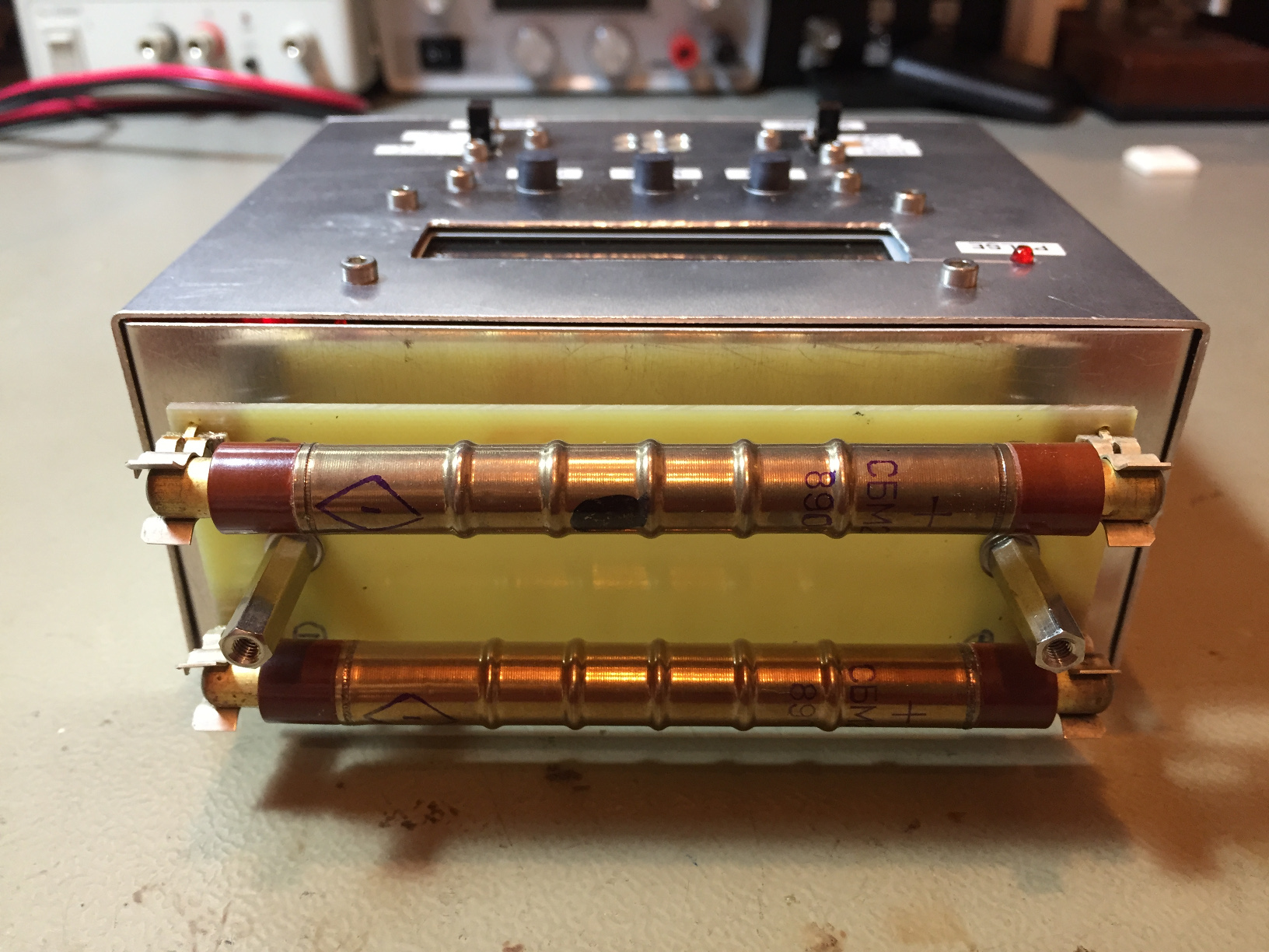
Front view of the instrument with and without protection cover (click
to enlarge).
I wanted the two Geiger tubes in the front, the display in the middle and the control switches at the back. To have good sensitivity, I mounted the tubes outside the main box. Geiger tubes are very fragile and care must be taken in handling them and in mounting them to the enclosure. First I wanted to fix them using a couple of zip-ties, but if too much pressure is applied, the 50 μm thick wall will bend and break, so I discarded this solution. I was also unsure if it was ok to solder directly to the tube terminals or not. Finally, I found that regular Ø 5 mm fuse holder clips work perfectly for this purpose: they hold the tubes by their terminals firmly and make a good electrical contact. So I prepared a piece of PCB with four fuse clips that I installed in the front. I didn't etch it: I just cut four islands with a cutter and peeled off the extra copper in-between.
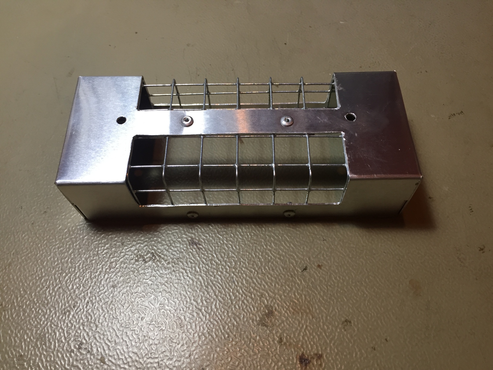
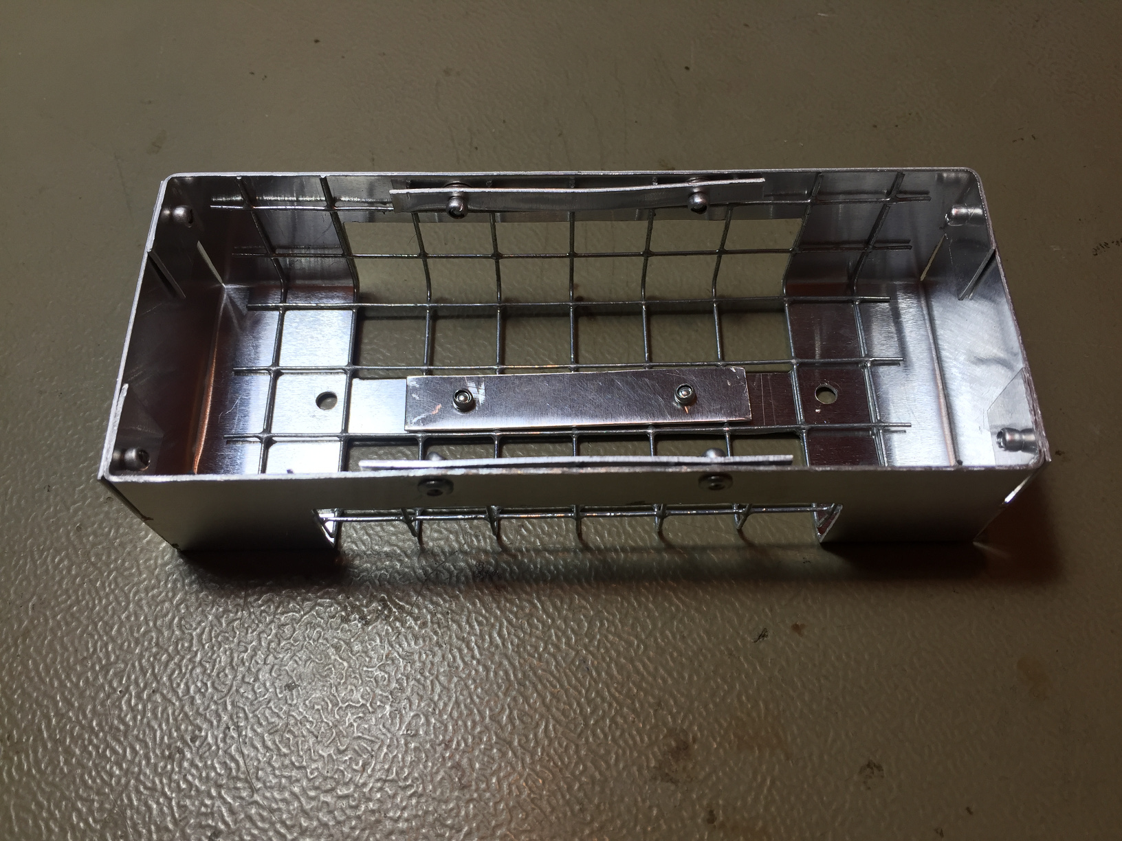
These two pictures show the protection cover intended to avoid
mechanical chocs on the tubes while letting radiation through (click to
enlarge).
To protect the tubes from external shocks, I made a dedicated cover with the same sheet aluminum. I cut two large windows that I covered with a 10 mm steel wire mesh to allow the radiation easily to reach the tubes. The first idea was to drill a lot of holes in the cover, but this leaves quite a large amount of metal in front of the tubes; the wire mesh is a much better solution because is about as strong but leaves the tubes almost unobstructed. Since this cover is external to the instrument, it's very easy to remove it, if extra sensitivity is needed.
A circuit that transforms radiation into pulses per minute is already a crude instrument, as it can directly be used to make relative comparison measurements. As long as we use the same instrument in the same conditions, we can compare the radiation of different samples or see if the values change over time.
But converting the pulses per minute into standard measurement units allows comparing with measurements done with other instruments or by different people. Unfortunately, I'm not a radiation expert and I don't fully understand the meaning of all the units used in this domain. So, I won't try to explain something I don't know... I'll simply explain what I have done and why: take it with skepticism and don't ask me questions, I don't know the answer.
Many old Geiger counters used to express their measurement in Röntgens per hour (R/h). In the SBM-20 datasheet, I found that it will generate 1'740 cpm when exposed to 1 mR/h of 226Ra and 1'320 cpm when exposed to 1 mR/h of 60Co. Not knowing which kind of radiation I may happen to measure, I simply took the average of these two values and I assumed that 1 mR/h of radiation will produce 1'530 cpm. I don't know how good this assumption is, but it's the best I could think of and gives a conversion factor to display readings in mR/h.
Later, I stepped upon another datasheet reporting the sensitivity of the SBM-20 tube for 137Cs, but only after having implemented and tested the instrument. Since I was already satisfied with the precision of the conversion factor I had, I decided not to change the value of 1'530 cpm per mR/h I was already using.
Now, many modern days counters use Sieverts per hour (Sv/h). I wasn't able to find any good (and simple) scientific document explaining how to convert the readings. According to [1], there are basically three main quantities: exposure, measured in Röntgens (R), adsorbed dose measured in Grays (Gy) or in rads (1 rad = 0.01 Gy) and dose equivalent measured in Sieverts (Sv) or in rem (1 rem = 0.01 Sv). I could also find in [1] that "if a (human) tissue is in a location exposed to 1 R, it will absorb about 1 rad". Also [2] agrees with this, stating that 1 mR/h is equivalent to 1 mrad/h. So 1 R corresponds to about 0.01 Gy and 1 R/h to 0.01 Gy/h. This is probably an approximation and I don't know what exactly the tradeoff is, but I couldn't find any better.
Both [1] and [4] say that the equivalent dose is calculated by multiplying the absorbed dose by the relative biological effectiveness (RBE), which is a dimensionless constant depending on the kind of particle and its energy. A Geiger counter is more or less sensitive to different particles and their energy, but will only generate pluses, regardless on the particle that was detected. So I don't know exactly how to select a suitable value for this constant. I could find in [2] two similar but slightly different equivalencies: 1 mrad = 0.877 mrem and 0.0869 mrem = 0.1 mrad. There are no explanation about why these two values are not the same, but the difference is about 1%, so I decided to arbitrarily select that 1 Gy = 0.874 Sv which is in-between. So, in summary, I assumed that 1 mR/h is approximately 8.74 μSv/h. From this, I could figure out that with this particular tube, 1 μSv/h should produce 175 cpm. Again, I don't know how good or reliable this conversion is in practical situations, but from the measurements I could perform, it looks pretty good. Maybe I just got lucky.
The biggest problem of this project is making sure it actually works. First, before attempting to measure any radiation, one has to make sure the circuit is fully functional. When the circuit is on, the background radiation should make it tick every few seconds. If not, try shorting one of the tubes (anode to cathode) with your fingers. You won't feel any shock as the current is limited by the 4.7 MΩ resistor, but every time you do that, the counter should tick.
Then, I disconnected the tubes and connected a TTL (0 to 5 V) pulse generator across R7: every pulse of the generator will make the counter tick. I set the pulse width (space) to 190 μs and tested different frequencies, from 1 Hz up to 5 kHz and checked that the microcontroller handled the pulses correctly and displayed the expected result. I repeated this test with the pulse generator across R8 getting the same results. Finally did the test one more time with the signal generator connected to both R7 and R8 to make sure the microcontroller correctly handles all the events even when they are simultaneous on both tubes.
Now the detector is measuring the background radiation and it would be nice to make sure the values it reads make sense. I don't have a calibrated source and not even a source at all. I don't even want one: it's dangerous after all. And I don't have a trustful calibrated meter I can use to compare my readings, neither. But the Swiss authorities maintain a network of detectors all across the country and their readings are available online [5]. So I selected one measuring station not too far from home and went there with my counter. I placed it as close as I could (say 2 meters apart) so that the measuring conditions would be very similar and I took an average reading for 15 minutes: I measured 108 nSv/h on my meter. Then I checked online the values of that particular station at that time and found 109 nSv/h: much better than expected for a homebrewed instrument where the only form of calibration is some values from unknown tube datasheets and some guessing on the conversion factors.
Since one measurement point is usually not enough, I decided to select another measurement station further away which has a different average reading and tried that one as well. This home built instrument measured 160 nSv/h and the data reported for that station was 157 nSv/h: another good measurement.
I know that such low radiation levels are below the inherent tube radiation specified in its datasheet and that I could just be measuring the radiation emitted by the tube itself. So, I took some measurements a second time at both places several months later: the counter consistently followed the radiation levels expected, lower at one place and higher at the other one, always within a few percent of the value reported by the official (and calibrated) detector. This makes me conclude that, at least at these low radiation levels, the counter is quite accurate and that the assumptions I took in determining the conversion factors are reasonable.
Even if this doesn't tell how this instrument will behave with significantly higher radiation levels, I don't have any better comparison opportunity and I don't want to take the risk of dealing with radioactive material, so I call this good enough for my purpose.
A Geiger counter is a device that counts incoming ionizing radiation particles in a given amount of time. The counts look and are random, only their average represents the intensity of the radiation. At first glance, it seems that the pulses are not uniform, sometimes they come all together, sometimes the counter is silent for several long seconds and it looks hard to get meaningful readings out of it. But some simple statistics can help in clarifying the situation. We know that each time a measure of the same sample is taken, the count is slightly different: what is the error on the measurements? And how long should I measure to have a good reading?
When a radioactive atom decays, it emits a particle: alfa, beta, beta plus, neutrons, and very often also gamma radiation. A Geiger counter can detect and count some of those radiations, but only a fraction of them because it doesn't have 100 % efficiency. When a decay will occur cannot be predicted: it's a pure random process. But there is a very very large amount of unstable atoms even in a small sample of material, each with a very low probability of decaying. All atoms are independent: the fact that one atom decays has no influence on the others. The average number of decays is constant or about constant during the measurement period: it's true that radioactive decays decreases with time, but half-life is usually much much longer than the time we need to take a measurement. If these conditions are met, and they usually are with Geiger counters, we can use the Poisson distribution, that says that all readings will be "bell-shaped" around the average (that we will call λ) and that the standard deviation is simply √λ. This is a powerful mathematical conclusion: we don't need to bother about the single readings and when they come, only their average counts.
Now, if the average is large enough (say greater than 10) we can approximate the Poisson distribution it with a Gaussian distribution of average λ and standard deviation √λ. In a Gaussian distribution, 68 % of the measurements are plus or minus one standard deviation around the average and 95 % are ±2 standard deviations around the average. With this we can easily calculate the error of the measurements.
I skip here the details of the math involved and the fact that we went from a discrete process (a pulse that arrives or not) to a continuous process (an average can very well be 17.5 pulses) but this is ok as long as the conditions explained before are met.
Let's take an example: suppose that we measure on average 100 counts every minute. The standard deviation will be √100 = 10. This means that 95 % of our readings are between in an interval of twice the standard deviation above and twice the standard deviation below the average. In other words, 95 % of the measurements will be between 80 and 120 cpm or, 100 cpm ±20 %.
Suppose now that we take a longer measurement with the same radioactive sample and we get 1'000 counts every 10 minutes. This is still 100 cpm, but the standard deviation is now √1'000 ≅ 31.6 counts. Here, 95 % of the readings are between 937 and 1'063 counts, in other words 100 cpm ±6 %. By taking a ten times longer measurements we increased the precision about 3 times.
Using the Poisson law is only allowed on the instrument counts, as they are the only thing that is Poisson distributed. As soon as you start manipulating the values by adding or subtracting them together or converting them into nSv/h or μR/h, using the statistics becomes much more complex and tricky. Please also remark that the integration time must not be taken into account in the average of our Poisson/Gaussian distribution; only the raw number of counts. If you take a longer measurement, you get a higher number of readings and therefore a more accurate result, but you don't divide by the time before calculating the statistics, you only do that after to make the units match.
This is probably the most important question. Unfortunately, I'm no radiation expert and I don't have a precise answer. But since I was interested in knowing if I have to worry about a potential high reading of my instrument, I did some research and I summarize in this section some values that I was able to find in the literature I had on hand. I just report them as they are: up to you to make your own opinion and to further investigate if needed. I also arbitrarily decided to use only printed documentation and do not use online data for this purpose; mainly because I have the feeling it's a more accurate source. It's just my choice here and there is nothing wrong about data available in the net; at the end, if you're reading this, you found it on the net anyway...
Both [1] and [4] report that a single exposure to a dose of less than 0.25 Sv (25 rem) has no short term clinical consequence, that exposures of 1 Sv (100 rem) have short term consequences (nausea, tissue damage,...) and that 5 Sv (500 rem) are lethal for 50 % of the exposed population in less than 30 days. But there are two important aspects that must be mentioned: first, this is related to a single, short (hours? days?) and very strong exposure and not to a constant exposure that will add to the same amount in one year. These are Sieverts, not nano-Sieverts! Second, these are only short term effects; long term effects (cancer?) that may appear years after the exposure are not excluded. This gives some reference in case of an exposure due to a major accident, but this is not the usual radiation you'll measure every day and is of little interest for this Geiger counter project.
For everyday exposure, it seems that there are two distinct thresholds: a higher one for workers in the nuclear industry and a lower one for normal population. I didn't investigate too deeply, this is a quite complex and vast topic: these thresholds are different for different countries, were changed several times over the years, have different values according to which part of the body is exposed and it's difficult to summarize a simple general rule. They are normally expressed in the total dose accumulated over one year. The idea is that one could absorb a slightly (reasonably) higher dose for a short period of time with no consequences if the total annual dose is not exceeded. Since Geiger counters usually give readings "per hour", I simply divided this dose by 8'766 (the total average amount of hours in one year), knowing that this dose could theoretically be slightly exceeded as long as the annual total stays below the threshold.
According to [1], nuclear industry workers should stay below 5 rem/y and normal population below 0.5 rem/y. Converted in nSv/h these thresholds are 5'700 nSv/h and 570 nSv/h respectively. According to [2], exposure (for normal population) should be below 600 mrem/y that corresponds to 680 nSv/h. I voluntarily expressed all these values in nSv/h even when μSv/h would have been more convenient, so that the figures are easier to compare without the need of doing the conversion while reading.
According to [5], usual values in Switzerland are normally between 80 and 260 nSv/h depending on the location. The place where the highest radioactivity is measured is in the Piz Guiv region (46° 42' 06.66" N, 8° 41' 33.21" E) where values up to 500 nSv/h have been recorded. I don't know about other countries.
Some commercial instruments produce an acoustic alert signal when the readings exceed a given threshold (this one doesn't). I've seen thresholds in the 600 to 2'000 nSv/h range according to the model and brand of the meter. I don't know how these thresholds are determined, but they look more or less consistent with the figures I reported above.
These values and thresholds are more a curiosity for me; it's just to have a rough idea of what radiation level is dangerous and what is normal. The Geiger counter described here is not calibrated in any way to any standard reference, so its measurements cannot be used to reliably determine if the radiation is precisely above or below a given threshold; still it gives a fair idea of the radiation in the environment.
In this page, the circuit of a simple twin-tube Geiger counter is explained. This is more in the attempt to give technical details of the development of interesting circuits rather than building a precise instrument. Special care is given for the design of the high voltage generator.
Of course a Geiger counter can be a useful tool if, one day, another nuclear disaster should happen. Having an instrument on hand to tell what is radioactive and by how much could help, even if I hope it will continue reading small values coming from a low background radiation only.
Again, I'm not a radiation expert or a nuclear physicist: consider this as an electronics project and not as a precise radiation measuring instrument. Also take the considerations and assumption on radiation, conversion factors and thresholds with skepticism.
| [1] | Paul A. Tipler. Invito alla fisica – 3. Zanichelli, 1992, "Dosimetria", pagine 859-863. |
| [2] | Come proteggerci dalle radiazioni nucleari. Nuova Elettronica, Anno 18, Numero 108/109, Luglio/Agosto 1986, Pagine 8-22. |
| [3] | LX.1407 – Un nuovo ed efficiente contatore Geiger. Nuova Elettronica, Anno 31, Numero 200, Giugno/Luglio 1999, Pagina 2. |
| [4] | T. L. Brown, H. E. LeMay Jr., B. E. Bursten, C. J. Murphy, P. M. Woodward, M. W. Stoltzfus, M. W. Lufaso. Chemistry: The Central Science (14th Edition), Pearson, New York, 2017, page 931. |
| [5] | Swiss National Emergency Operation Centre. Radioactivity, www.naz.ch 2017. |
| [6] | S. Rozsa. Nuclear measurements in industry, Elsevier, Amsterdam-Oxford-New York-Tokyo, 1989, section 2. |
I was unable to find an official complete datasheet in English for the SBM-20 tube. Actually, I wasn't even able to figure out who is manufacturing these tubes and if they are still produced today. I found several different scanned documents in Russian which I don't fully understand and some translations that do not correspond perfectly. Here is a summary (compilation) of all the data I was able to collect from various online sources. I don't report here the exact references for these sources, as they come from unofficial websites like personal webpages (like this one) or online auction sites that are very likely to disappear or to be moved in the near future. Many of them already have and a broken internet link is of no use. Because the data comes from different sources on the web and not from the original manufacturer, take it with skepticism even if it worked perfectly for this design. If you need trustful and reliable data, try searching the internet again, maybe you'll be luckier than me.
| Mechanical characteristics | |
| Overall length: | 108 mm ±1 mm |
| Overall diameter: | 11 mm +0.2 mm−0.5 mm |
| Weight: | 10 g |
| Cathode wall material: | Stainless steel |
| Cathode wall thickness: | 50 μm |
| Wall density: | 40 mg/cm2 |
| Maximum external pressure: | 1.5 kgf/cm2 |
| Operating temperature range: | −60 °C ... +70 °C |
| Gas filling: | Ne, Br2, Ar |
| Electrical characteristics | |
| Operating voltage range: | 350 V ... 475 V |
| Recommended operating voltage: | 400 V |
| Plateau length: | > 100 V |
| Maximum plateau slope: | 0.1 %/V |
| Maximum DC current: | 20 μA |
| Minimum anode resistor: | 1.0 MΩ |
| Recommended anode resistor: | 5.1 MΩ |
| Pulse amplitude: | > 50 V |
| Insulation resistance: | > 1 GΩ |
| Tube Capacitance: | 4.2 pF |
| Maximum dead time: | 190 μs (at 400 V) |
| Tube life: | > 2·1010 pulses |
| Sensitivity | |
| Ionizing radiation type: | Gamma and hard beta |
| Working range: | 0.004 μR/s ... 40 μR/s (0.014 mR/h ... 140 mR/h) |
| Gamma sensitivity (226Ra): | 420 cps ±20 cps at 4 μR/s (29 cps/(mR/hr)) |
| Gamma sensitivity (60Co): | 315 cps at 4 μR/s (22 cps/(mR/hr)) |
| Gamma sensitivity (137Cs): | 240 cps ... 280 cps at 4 μR/s (18 cps/(mR/hr)) |
| Inherent tube background: | < 1 cps |
| Home | Electronics | Page hits: 022755 | Created: 12.2017 | Last update: 12.2017 |