This article describes a method to match short antennas to standard transmission lines. It's mainly intended for radio amateurs working on 137 kHz and 500 kHz bands, because when dealing with long waves, matching the antenna is always a problem. Traditional matchboxes designed for short waves do not have enough capacitance and inductance to work on low frequencies, and large commercially available variable capacitors and inductors are expensive and hard to find. Furthermore, installing an appropriate antenna, let's say a quarter wavelength tower, is out of reach for the common amateur. So, all long wave ham antennas are always too short and are a nightmare to match to a 50Ω line.
What one usually does is trying to run a wire as long as possible as high as possible. Any short antenna can be matched with this method, such as towers with or without capacitive hat, T antennas, inverted-L antennas, random wires, and so on, as long as they are small compared to the wavelength; shorter than a quarter wavelength in any case. Let's imagine one wire going vertically for 8 meters and than horizontally for 45, and take this antenna as an example, as shown in the figure below.
This is already a big antenna for a backyard, but really small compared to the 2200 m (600 m) wavelength of the 137 kHz (500 kHz) band.
The impedance of an antenna can be simulated with a NEC based program by "drawing" and approximating its structure and four our example the results are as follows:
| Simulation frequency |
Antenna impedance |
Equivalent capacitance |
Radiation resistance |
| 137 kHz | (0.7 – j3900) Ω | 298 pF | 0.01 Ω |
| 500 kHz | (1.4 – j960) Ω | 330 pF | 0.12 Ω |
The impedance has a very low resistance in series with a very high capacitive reactance which is typical of short antennas and the results look plausible.
If the antenna cannot be simulated, one can still build an antenna as high and as long as possible and then measure the static capacitance. Since we are far below the first resonance, the antenna will look like a capacitor, and with some luck we can measure its static capacitance with a capacitance meter. Please remark that unfortunately some capacitance meters use a too high frequency and gives inconsistent results: in order to be accurate, the frequency should be as low as possible, but definitively not higher than the design frequency (the antenna has to be short at the measuring frequency). Connecting a capacitance meter to the antenna taken as example gives 295 pF; not far from the simulated values and the static capacitance is a really good starting point.
Another method to measure the static capacitance of the antenna is to connect an inductor of known value in parallel to its feed point and to measure the resonance frequency. Again, this frequency has to be as low as possible to make sure the antenna is still "short" and a large inductor must be used. Once the capacitance has been determined, the capacitive reactance can be easely calculated with the formula Xc = 1/(2πfC).
The two above described measuring methods only determine the capacitive reactance but not the resistance. It's pretty hard to measure values as low as a few ohms while having kiloOhms of reactance in series, but knowing the exact real part of the impedance is not really important, since this will have little effect on the design of the match, as we will see later. Assuming just one or two Ohms is accurate enough.
So, the antenna looks like a big capacitor with a small resistor in series, which we would like to transform in purely resistive impedance Zc, let's say 50 Ω with a matching network. If we plot the antenna impedance Za on the complex plane, we find a point very close to the vertical axis, much lower than the horizontal axis. Zc is of course located on the horizontal axis on the right, as one can see in the figure below:
The goal is to reach Zc starting from Za as shown by the dashed line. No component can achieve this in one step and we will match the impedance in two steps.
We have several choices: if we connect a series capacitor Cs to the antenna, a parallel inductor Lp or a step down transformer N:1 (more turns on the transmitter side), Za will be transformed in a higher impedance (we are moving away from the origin) and this situation must be avoided because a high impedance means a high voltage, much higher than the already high voltage typical of a short antenna. Let's imagine to connect a 1 kW transmitter on our antenna at 137 kHz: with an impedance around 3900 Ω the voltage on the feed point will be 2 kV! This is already high enough to make some trouble and we definitively don't want to deal with higher voltages in the matching network.
If we connect a parallel capacitor Cp or a step up transformer 1:N (more turns on the antenna side), Za will be transformed in a lower impedance (we are moving towards the origin) and this situation must be avoided because this reduces both the reactance and the resistance. The resistance of a short antenna is already very low (in the Ohm range), reducing it will dramatically increase the losses in the matching network and this ahs to be avoided as well.
So, the only choice is to connect a series inductor Ls to the antenna in order to reduce ("resonate away") the huge capacitive reactance of the antenna without reducing the resistive part of the impedance. In the figure this means moving vertically in the up direction. It's good to remark that the best choice is also consistent with common sense, as one would most probably think in matching a capacitive load with a series inductor.
Now that we determined that the first element of the matching network is a series inductor Ls connected to the antenna, we have to determine the second element that will finish the match.
As it can be seen in the figure above, here we have three choices. The first idea is to resonate away completely the capacitive reactance with Ls and find the intermediate impedance Zi2 which lays in the real axis and than use a step down transformer N:1 (more turns on the transmitter side) to reach Zc. This solution could work but requires a transformer which takes longer to build, adds some difficulties to the design and requires more copper and has therefore higher losses.
The second possibility is to over-compensate the capacitive reactance of the antenna with a slightly larger series inductor Ls reaching point Zi3 which is slightly inductive and lays on the constant admittance circle passing through Zc. Using a parallel capacitor Cp we can reach Zc. This solution can work as well and good capacitors have very little losses, but the capacitance required is very large. In order to match the antenna of our example at 137 kHz some 200 nF are required: not easy to find and not easy to adjust as variable capacitors are usually in the few 100 pF range.
The third and preferred option is to slightly under-compensate the capacitive reactance of the antenna with a slightly smaller series inductor Ls reaching point Zi1 which is slightly capacitive and lays on the constant admittance circle passing through Zc. Using a parallel inductor Lp we can reach Zc. This solution has several advantages: first it requires only a small parallel inductor; it has the shortest path between Za and Zc (meaning low losses) and is easier to build.
So, after having analyzer the different options we have determined that the impedance follows the path shown in the plot below:
With a series inductor Ls connected at the antenna port and a parallel inductor Lp connecter at the transmitter port. Our matching network looks like the following diagram:
Now, to determine the value of the two inductors, one can use the two equations above and with our antenna we get:
| Frequency | Antenna impedance |
Series reactance |
Parallel reactance |
Series inductor |
Parallel inductor |
| 137 kHz | (0.7–j3900) Ω | 3894 Ω | 6.0 Ω | 4.5 mH | 6.9 μH |
| 500 kHz | (1.4–j960) Ω | 952 Ω | 8.5 Ω | 300 μH | 2.7 μH |
In order to simplify this operation the following calculator can be handy:
Just enter the working frequency f, the transmitter impedance Zc (usually 50 Ω), the antenna impedance Za and hit the button to calculate the required series and parallel inductances Ls and Lp.
To calculate the required number of turns, an empirical formula that works well is described in the ARRL Handbook. Transformed for metric units is as follows:
 |
 |
Where d is the diameter in mm, l is the length in mm and N is the number of turns. The calculated inductance L is in μH. When designing a large coil, it's more practical to use the turns spacing s in mm than the total length. s is defined as l/N.
In order to simplify coil design, the following calculator can be handy:
Just enter the core diameter d, turns spacing s, the desired inductance L and hit the "Calculate N" button to computer the number of turns N and the overall coil length l. As verification, one can enter the number of turns N and hit the "Calculate L" button to compute the inductance L and the overall coil length l, based on the same diameter d and spacing s.
The values we have just calculated are approximate since are based on simulations, on low precision measurements, on arbitrary assumptions and on a simplified theoretical model. Therefore real inductors require some adjustment and must be variable. Changing the transmit frequency inside the band requires retuning as well. Experience shows that only Ls needs adjustment, Lp is less sensitive to frequency changes and once tuned can stay fixed for the whole band.
There are several ways to make a variable inductance and the easiest is to change the number of turns. One could wind a coil with more turns than needed and than make connections to intermediate taps, as shown in the figure below.
There is always debate about shorting unused turns or not (the dashed line in the figure). Shorting them results in higher losses while leaving them open may result in high induced voltage and arcing. As we will discuss later, in an air core solenoid the coupling factor between the turns is low and doesn't work well as autotransformer; on the other hand if the unused coil section happens to be resonant at the working frequency high voltage may result. This is quite unlikely since the working frequency is low and fairly fixed; a resonance requires significant stray capacitance which is unlikely with a small coil section. It's therefore wiser to leave unused turns open reducing losses unless arcing takes place leaving no other choice than shorting them. If the unused turns have to be shorted it's better not to short them all but to leave a small gap to let the field "escape", as shown in the figure below:
Another way to have a variable inductor without involving too much mechanics is to build a variometer as summarized below:
The coil is split in half and a smaller coil is inserted inside the first one and connected in series. By turning the small coil inside it's possible to increase the total inductance (when both coils are aligned in phase) or to decrease it (when both coils are aligned with opposite phase). A variometer has higher losses because the wire is longer, but on the other hand it's easy to build and has no sliding contact.
The final solution is to use a tapped coil for Lp and a variometer for Ls. Lp is small and is not adjusted frequently, usually on once when the antenna is first tuned, so a tapped coil is acceptable. Ls needs to be adjusted every time the working frequency is moved, even a few hundred Hz, making the variometer solution more practical because of its continuously adjustable value.
A variometer is easy to build with readily available materials. Two plastic pipes of different diameters, insulated copper wire and a plastic rod for the shaft are the main components. The figure below shows the cross section and the way the coils are connected together.
Whit the formula (or the calculator) we discussed before, on determines the required number of turns on the external (stator) coil. This coil is split in two to let same space for the shaft to cross the core. A second coil, small enough to turn inside, is built and connected to the shaft and forms the rotor. All inductors are connected in series. Since the rotor only needs to move 180°, there is no need for sliding contact since flexible wire will do nicely the job.
It's hard to determine exactly the range of variation of the inductance of a variometer, since this strongly depends on the coupling factor between stator and rotor coil, but as a rule of thumb, the experience shows that the total inductance will be something in-between Lstat±Lrot and Lstat±2Lrot and is a fair starting point. The best swing is obtained when all the coils are symmetrical. If the variation happens to be too small, one can still add a second layer of turns on the rotor.
A question still remains: do we really need two separate inductors? Well, theoretically yes, the two inductors need to be separate and not coupled at all. On the other hand, if we talk about air core solenoids, the answer may be yes under certain conditions. In an air core solenoid, the coupling between turns is fairly low and further decreases as the distance between the turns increases. It's therefore possible to wind on the same core both Ls and Lp, adjacent to each other. The whole matching network looks than as an autotransformer, but it's not (or it's a very bad one), as explained later. Lp can be adjusted by selecting a suitable tap on the main coil and Ls can be adjusted by turning the variometer. This works only if the coupling factor is low: meaning that there is no magnetic core inside the coil, the turns are on only one layer in proximity of Lp (coupling factor is much higher for two windings one inside the other)the variometer inside Ls is far from Lp, and Lp is small compared to Ls.
The final antenna tuner looks like the above diagram. This really looks like an autotransformer, but it's not really one. If it was an autotransformer it could not cancel the reactive component of the impedance. The antenna could not be matched, since it will just transform down the complex impedance of the antenna into another smaller complex impedance, something like (0.01–j50) Ω, but to match the antenna it's necessary to remove the reactance and to transform the resistance to 50 Ω. Just adjusting one parameter is not enough: the matching network must transform both.
On the other hand, if we imagine that part of the coil works like an inductance, cancelling out the reactive part of the antenna impedance, the rest of the coil cannot be an autotransformer either, because once the reactance has been resonated away, the impedance is real and very low. It would require a step-down transformer (more turns on the transmitter side) instead of a step-up transformer, which is how the antenna tuner looks like.
In order to check the coupling between the turns and the autotransformer effect, the setup shown in the figure below has been built:
The coil has a diameter of 200 mm, a length of 280 mm, 100 turns and a tap on the 4th turn. The transformer turn ratio is therefore 1:25. A voltage Up of 1 Vpp has been applied on the 4 turns and the voltage across the whole 100 turns Us has been measured. Several measurements were taken at different frequencies and show that for this the voltage Us is around 4 Vpp from a few kHz until about 400 kHz. The transformer ratio is therefore 1:4, very far from the expected 1:25, meaning that only the first few turns are coupled and that the rest of the coil is just an inductor. In this case, if the frequency is increased to 463 kHz we have a resonance and Us goes up to 55 Vpp, much more than what a 1:25 step-up transformer would do. Further increasing the frequency lowers Us down again to 4 Vpp until other resonances occurs.
It's best to think of this antenna tuner as two separate inductors, one in parallel with the transmitter and the other in series with the antenna, but because of the coupling between the two, the required values will be slightly different, especially for the small Lp, but this it's not a big issue, since, it's just a matter of finding the correct tap on the coil.
Now that we have determined how our antenna tuner will be and how many turn we'll have to wind, let's spend a few words about the construction. First of all, we should try to design a tuner with minimal losses, but this is not an easy task. The wire used to wind the coils will be responsible for the majority of the losses and choosing a large diameter wire is a good idea. "Litz" wire is definitively the best option, but this is almost impossible to find in large diameters. The second preferred option is enameled copper wire, which is easier to find but expensive. The third option is to use PVC insulated electrical installation wire. This wire is relatively cheap, easy to find and available in large diameters. There is one detail one should take care of: the copper must look "red" and not be tinned. Tinned wire has very high losses at radio frequency and should be avoided. PVC insulation is not the best option because of its poor tg(δ), but the frequency is low and can be accepted; Teflon isolation would be a better option.
Concerning the core, the best core is no core at all, but this won't be possible for such a big coil. Ceramic cores are very, but very hard to find in large sizes, so the third option is to use PVC pipes. These pipes are available in many large diameters, are cheap and are easy to work. They are a bit lossy, but again, the frequency is low and can be accepted for amateur use.
In short antennas, the resistive part of the impedance is highly dominated by losses. Trying to reduce losses is always a good idea. For example one could use a few (or more) buried radials to increase ground conductivity near the antenna (where the current is higher). Another idea is to use more than one aerial conductor running parallel at some distance apart: this will split the current and reduce the losses.
Using this antenna tuner is quite easy: since the topology of the matching network has only two parameters to adjust, there is no risk to find a "wrong" and lossy match.
If one happens to have an antenna analyzer that works at the desired frequency, this is by far the best option to adjust the tuner. If not, just connect the antenna and the transmitter (with a suitable SWR meter) and select low power operation. Adjust the variometer first is to find the position where the SWR is the lowest, then move the tap between Ls and Lp to find the best possible match (don't forget to switch the transmitter off before moving the tap). There is nothing more to do as this will usually allow match as good as 1.2:1 if there are enough taps. If the match is not good enough, try to repeat these two operations again maybe adding some more intermediate taps to the coil. If frequency is changed, usually only the variometer needs to be adjusted again and the tap can stay fixed for the whole band.
Please remark that the majority of SWR meters designed for short-waves operations do not work for long waves. One should check before with a 50 Ω dummy load if the instrument gives reasonable results at the desired frequency.
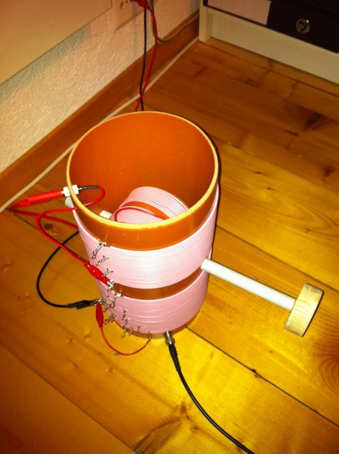
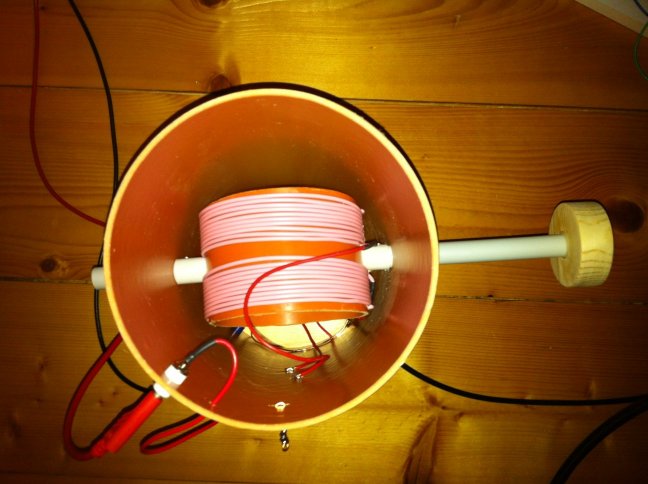
The above described matching networks have been built and tested. The following pictures show a variometer designed for the 137 kHz band. The main coil can be adjusted between 3.75 and 4.63 mH and matches the antenna used as example at 137.3 kHz with an inductance of 4.39 mH. We can therefore calculate the capacitance of the antenna in 306 pF. In order to achieve the required inductance with less wire, some additional turns have been added inside the main coil (on the opposite side of Lp). The rotor of the variometer is also a double layer coil. The loaded Q of this matching unit (loaded with the antenna) is about 60.
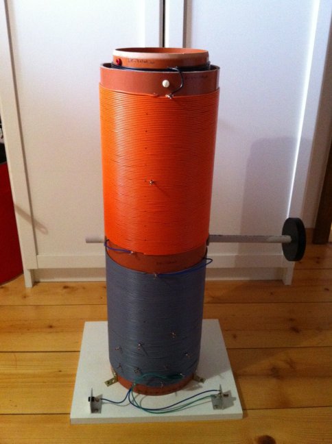
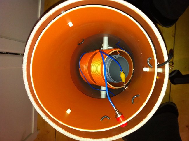
The second variometer is designed for the 500 kHz band and can be adjusted from 214 to 598 μH by moving the variometer and selecting one of four taps on the upper side of the coil. It matches the same antenna at 500 kHz with 288 μH and we can calculate the capacitance at this new frequency in 352 pF. The loaded Q of this antenna tuner is about 80.
A simple way of matching an electrically short antenna to a standard 50 Ω transmission line has been explained. Both theoretical and practical aspects have been addressed. The goal is to help radio amateurs in tuning their (short) antenna with the hope that more and more hams will be interested in medium and long wave frequency bands.
| Home | Electronics | Page hits: 068674 | Created: 11.2011 | Last update: 11.2011 |